Original paper: Ultrafast reversible self-assembly of living tangled matter
Author: Sri Ganesh Subramanian
Editors: Jack Llewellyn, Manikuntala Mukhopadhyay
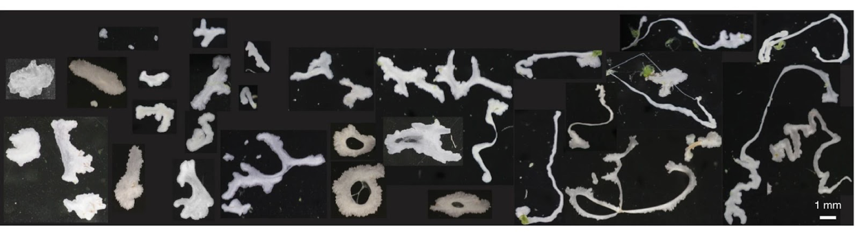
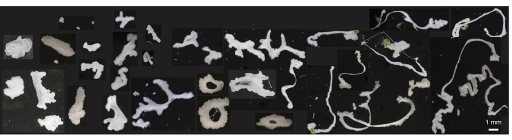
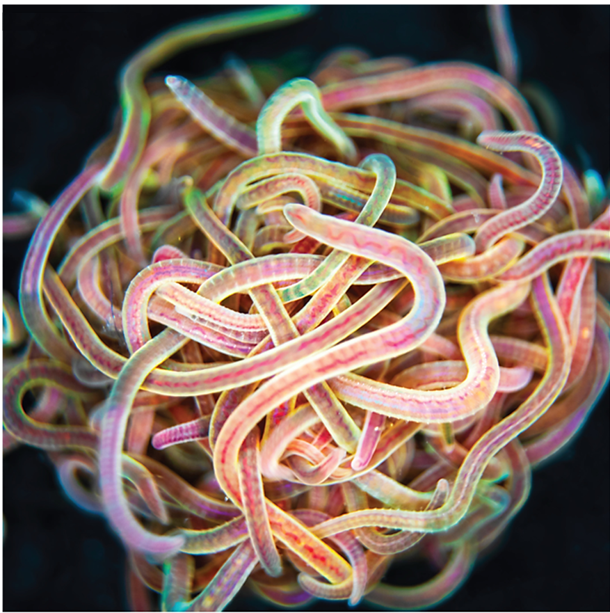
Many of us would have tied several knots very easily, but we all remember the frustration when trying to untangle the cords of a headphone – an experience that often tests our patience. Now imagine a creature that not only creates a tangled ball out of itself and its companions in minutes but can also untangle the entire knot in milliseconds if it senses danger. Meet the California blackworm (Lumbriculus variegatus), a small yet remarkable organism that is teaching researchers innovative lessons about managing tangles (see Figure 1).
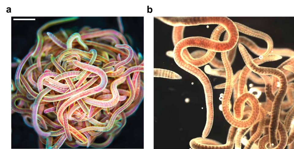
At first glance, studying the movement of worms might seem unusual or even unpleasant. However, researchers in the Bhamla Lab at Georgia Institute of Technology and Massachusetts Institute of Technology, USA, were captivated by the rapid untangling behavior of these worms. The scientists noticed that these worms naturally tangle together for survival. By assembling themselves in the shape of a compact ball, they reduce water loss, regulate temperature, and protect themselves from environmental challenges. Their most astonishing trait, however, is their ability to instantly untangle (within a few milliseconds) and scatter in random directions when they feel threatened. Scientists are studying these worms to uncover how their movements enable them to form and break apart tangles so efficiently, and how these principles can be applied to develop innovative materials and technologies.
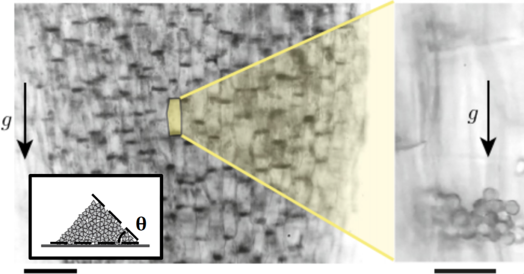
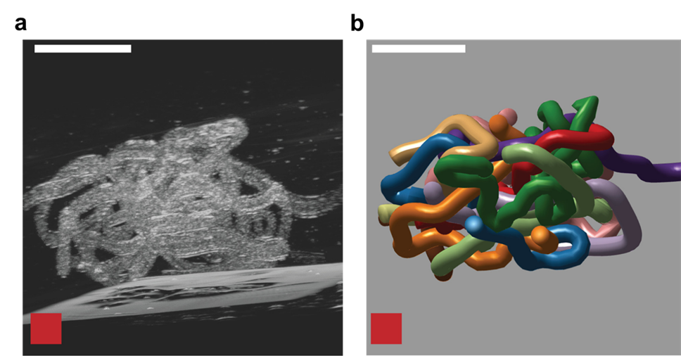
To understand how blackworms form and break tangles, scientists used ultrasound imaging to look inside these clusters. Because blackworms untangle almost instantly when disturbed, the researchers needed a method to slow their movements without harming them. The scientists carefully submerged the worms in a glycerol bath (a non-toxic viscous liquid commonly used in products like chewing gums and marshmallows) at a controlled temperature, to reduce their speed (Figure 2a). After allowing the worms to settle in the glycerol bath, the researchers carefully directed ultrasound waves from multiple directions to track the position of these worms as they moved over one another. This allowed the researchers to create a 3D image of the worms in their tangled state (Figure 2b). What they found was surprising: the tangles aren’t random. The worms were tightly packed, and most of them were in contact with one another, forming an intricate and highly organized structure.
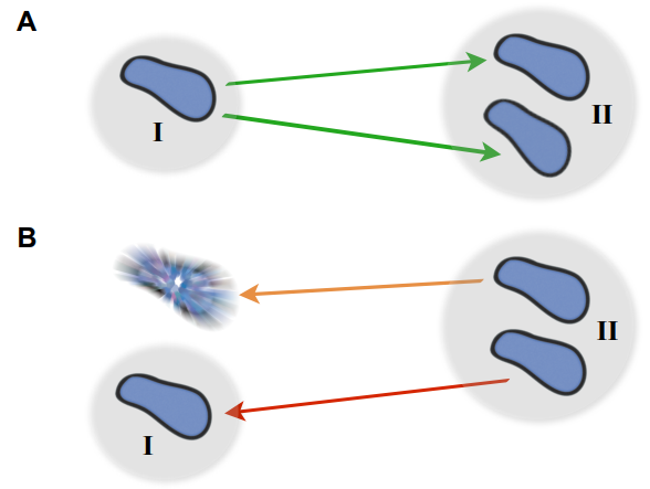
By analyzing how the worms moved and interacted, researchers identified specific patterns that dictate how these tangles form and function. They discovered that each worm’s position and movement contribute to the overall structure. Additionally, the size of the tangle could range from a handful of worms to several hundred, depending on environmental conditions and the size of the group. The researchers also discovered that the movements of the worms are critical to their tangling abilities. To tangle, the worms moved slowly and created loops that naturally intertwine. Over time, these loops formed a dense and stable structure. Untangling, however, is a completely different process. When blackworms sense danger, they generate rapid, wave-like motions through their bodies known as helical waves. These waves act like a zipper being undone, loosening the knots and allowing the worms to quickly break free, within a few milliseconds.
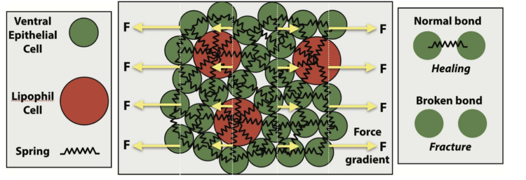
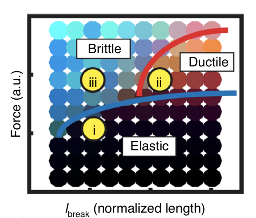
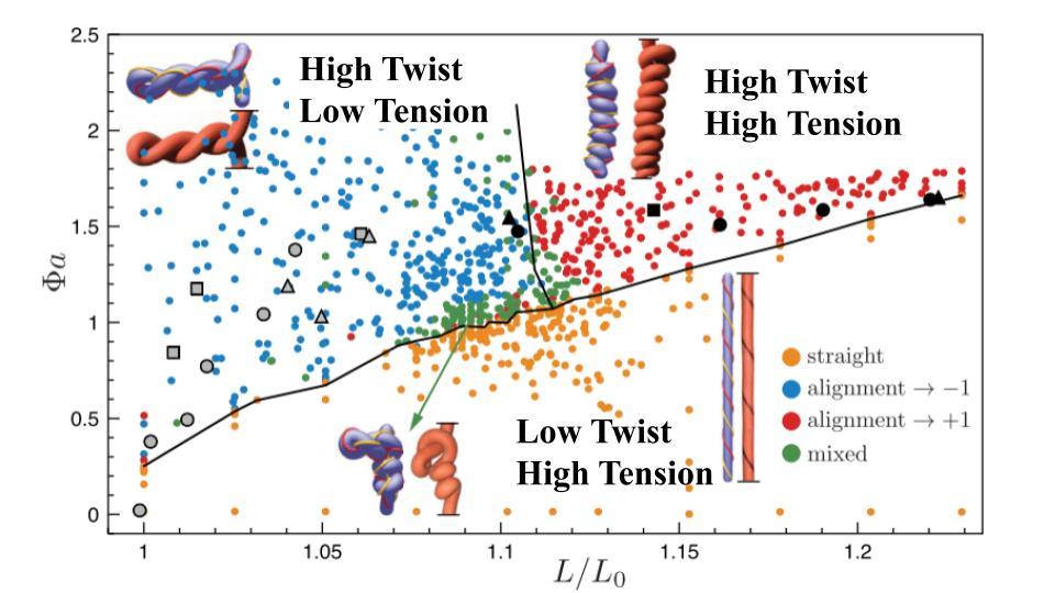
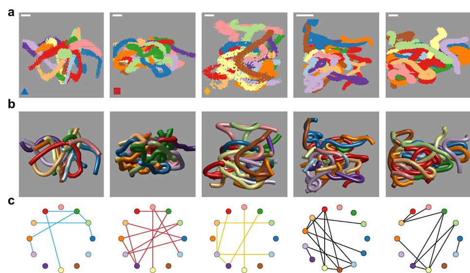
To better understand these motions, researchers created mathematical models to understand how the movement of the worms lead to tangling and untangling. The models showed that factors such as speed, direction, and frequency of the worms’ movements are precisely tuned to achieve their goals with remarkable efficiency. One of the most exciting outcomes of this research is the creation of a “tangle map” (see Figure 3). This map identifies the factors that influence whether worms tangle or untangle. These factors include movement speed, the angles at which the worms twist, and how often they change direction. By manipulating these variables, the worms can control whether they form a strong tangle or quickly break free and disperse.
This map also helps scientists understand how to replicate these behaviors in synthetic materials. For instance, by mimicking the worms’ twisting and untwisting motions, engineers could design materials that assemble and disassemble in response to environmental factors, such as temperature changes or mechanical stress. For example, in disaster response scenarios, robots inspired by blackworms could navigate through rubble by tangling and untangling themselves to squeeze into tight spaces. Similarly, materials that adapt to different conditions could improve everything from clothing to architecture. Blackworms remind us that sometimes the solutions to our most complex challenges are hidden in the simplest of creatures.
Disclosure: The author declares no competing interest.