

Original paper: Growth and division of active droplets provides a model for protocells
In the beginning there was… what, exactly? Uncovering the origins of life is a notoriously difficult problem. When a researcher looks at a cell today, they see the highly-polished end product of millennia of evolution-driven engineering. While living cells are not made of any element that can’t be found somewhere else on earth, they don’t behave like any other matter that we know of. One major difference is that cells are constantly operating away from equilibrium. To understand equilibrium, consider a glass of ice water. When you put the glass in a warm room, the glass exchanges energy with the room until the ice melts and the entire glass of water warms to the temperature of the room around it. At this point, the water is said to have reached equilibrium with its environment. Despite mostly being made out of water, cells never equilibrate with their environment. Instead, they constantly consume energy to carry out the cyclic processes that keep them alive. As the saying goes, equilibrium is death[1]: the cessation of energy consumption can be thought of as a definition of death. The mystery of how non-equilibrium living matter spontaneously arose from all the equilibrated non-living stuff around it has perplexed scientists and philosophers for the better part of human history[2].
An important job for any early cell is to spatially separate its inner workings from its environment. This allows the specific reactions needed for life, such as replication, to happen reliably. Today, cells have a complicated cell membrane to separate themselves from their environment and regulate what comes in and what goes out. One theory proposes that, rather than waiting for that machinery to create itself, droplets within a “primordial soup” of chemicals found on the early Earth served as the first vessels for the formation of the building blocks of life. This idea was proposed independently by the Soviet biochemist Alexander Oparin in 1924 and the British scientist J.B.S. Haldane in 1929[3]. Oparin argued that droplets were a simple way for early cells to separate themselves from the surrounding environment, preempting the need for the membrane to form first.
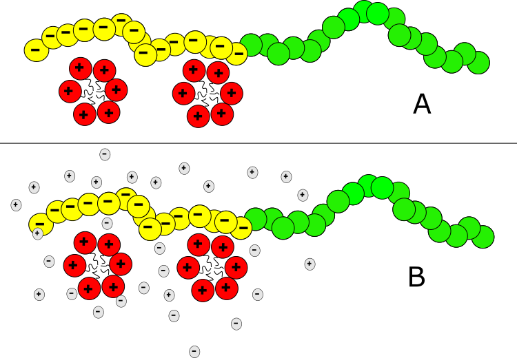
In today’s paper, David Zwicker, Rabea Seyboldt, and their colleagues construct a relatively simple theoretical model for how droplets can behave in remarkably life-like ways. The authors consider a four-component fluid with components A, B, C, and C’, as shown in Figure 1. Fluids A and B comprise most of the system, but phase separate from each other such that a droplet composed of mostly fluid B exists in a bath of mostly fluid A. This kind of system, like oil droplets in water, is called an emulsion. Usually, an emulsion droplet lives a very boring life. It either grows until all of the droplet material is used up, or evaporates altogether. However, by introducing chemical reactions between these fluids, the authors are able to give the emulsion droplets in their model unique and exciting properties.
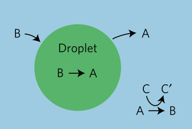
The chemical reactions in the model are fairly simple (see figure 1). Fluid B spontaneously degrades into fluid A and diffuses out of the droplet. While fluid A cannot easily turn back into fluid B (since spontaneous degradation implies going from a high energy state to a low one), fluid C can react with A to create fluids B and C’, and this fluid B can diffuse back into the B droplet.
$latex B \to A \quad \text{and} \quad A+C \to B+C’$
If C and C’ are constantly resupplied and removed, respectively, they can be kept at fixed concentrations. Without C and C’, the entire droplet would disappear by degrading into fluid A, reaching equilibrium. Here, C and C’ act as fuel that constantly drives the system away from equilibrium, creating what the authors dub an “active” emulsion. Active matter systems like this one have had success in describing living things because they, like all living matter, fulfill the requirement of being out-of-equilibrium.
Because the equations that describe how fluids A and B flow over time are so complicated, the authors solve their model using a computer simulation. When they do, something remarkable happens. Emulsions with no chemical reactions with their surrounding fluids never stop growing as long as there is more of the same material nearby to gobble up. This process is called Ostwald ripening[4]. The authors find that an active emulsion system, due to the fact that material is constantly turning over, suppresses Ostwald ripening and allows the emulsion droplet to maintain a steady size.
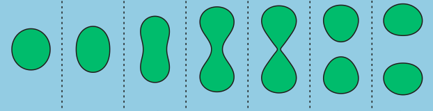
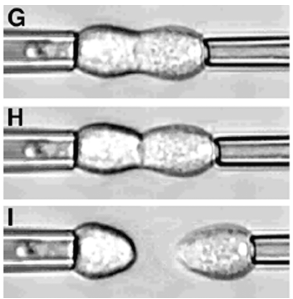
In addition to limited growth, the authors also find that the droplets undergo a shape instability that leads to spontaneous droplet division (see this movie). This occurs due to the constant fuel supply of C and C’. The chemical reaction A+C ? B+C’ creates a gradient in the concentration of fluids A and B outside the droplet. Just outside the droplet, there is a depletion of B and an abundance of A, while far away from the droplet, A and B reach an equilibrium concentration governed by the rate of their reactions with C and C’. The authors dub this excess concentration of B far away from the droplet the supersaturation. Where there exists a gradient in the concentration of a material, there exists a flow of that material, called a flux. This is the reason a puff of perfume in one corner of a room will eventually be evenly distributed around that room. The size of the droplet is dependent on the flux of fluid B into and out of the droplet.
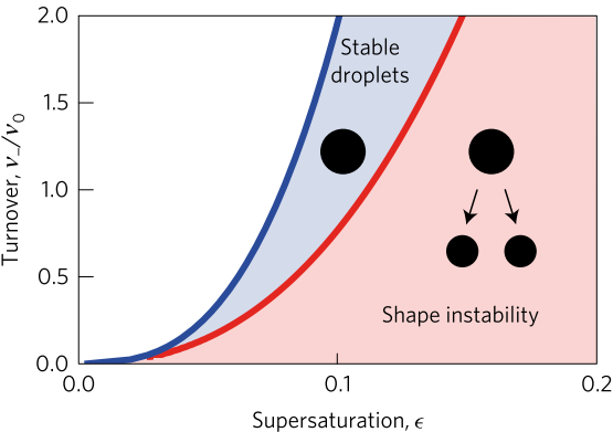
Two quantities determine the evolution of the droplet. The first is the supersaturation that reaches a steady value once all fluxes stop changing in time, and the second is the rate at which the turnover reaction B?A occurs. For a given supersaturation and turnover rate, the authors can calculate how large the droplet will grow, and they find three distinct regimes. In one regime, the droplet dissolves and disappears as the turnover rate outpaces the flow of fluid B back into the droplet. Another has the droplet grow to a limited size and remain stable, since the turnover and supersaturation balance each other out and give a steady quantity of fluid B. The third and most interesting regime occurs if the droplet grows beyond a certain radius due to the influx of fluid B outpacing its efflux. Here, a spherical shape is unstable and any small perturbation will result in the elongation and eventual division of the droplet (Figure 2).
And that’s it. If you have two materials that phase separate from each other, coupled to a constant fuel source to convert one into the other, controlled growth and division will naturally follow. While these droplets are more sophisticated than regular emulsion droplets, they are still a far cry from even the simplest microorganisms we see today. There is no genetic information being replicated and propagated, nor is there any internal structure to the droplets. Further, the droplets lack the membranes that modern cells use to distinguish themselves from their environments. An open question is whether a synthetic system exists that can test the model proposed by the authors. Nevertheless, these active emulsions provide a mechanism for how life’s complicated processes may have gotten started without modern cells’ complicated infrastructure.
Though many questions still remain, Zwicker and his colleagues have lent considerable credence to an important, simple, and feasible theory about the emergence of life: it all started with a single drop.
[1]: This isn’t exactly true. Some organisms undergo a process called anhydrobiosis, where they purposefully dehydrate and rehydrate themselves to stop and start their own metabolism. Also, some bacteria slow their metabolism to avoid accidentally ingesting antibiotics in a process called “bet-hedging”.
[2]: For example, ancient Greek natural philosophers such as Democritus and Aristotle believed in the theory of spontaneous generation, eventually disproven by Louis Pasteur in the 19th century.
[3]: Oparin, A. I. The Origin of Life. Moscow: Moscow Worker publisher, 1924 (in Russian), Haldane, J. B. S. The origin of life. Rationalist Annual 148, 3–10 (1929).
[4]: Ostwald ripening is a phenomenon observed in emulsions (such as oil droplets in water) and even crystals (such as ice) that describes how the inhomogeneities in the system change over time. In the case of emulsions, it describes how smaller droplets will dissolve in favor of growing larger droplets.


