Original paper: Sodium Dodecyl Sulfate (SDS)-Loaded Nanoporous Polymer as Anti-Biofilm Surface Coating Material
Are you afraid of visiting the dentist? If so, you’re probably not the only one, but unfortunately we can’t avoid it. Yearly dental check-ups are necessary to prevent tooth and gum infections. Dentists use a disturbingly sharp, noisy tool to remove dental plaque from the tooth surface. Dental plaque is caused by bacteria, and it is an example of a biofilm, which is a community of bacterial cells that stick to surfaces. Biofilms can be found everywhere, especially on wet surfaces. Biofilms cause health problems for millions of people worldwide every year, primarily because of infections during surgery or consumption of contaminated packaged foods. To prevent these problems, some scientists are developing surface coatings that will prevent biofilm formation in the first place. In this week’s paper, we will learn about a new technique for creating a microscopic “shield” against the formation and growth of biofilms.
A biofilm is a complicated microscopic world in which multiple bacterial species can coexist. Most parts of the biofilm are covered by a protective sticky slime that is produced by the bacteria themselves. It is now known that bacteria communicate with each other within the biofilm by exchanging small molecules, proteins, genes, and even electrical signals. This intercellular communication results in expression of specific genes throughout the bacterial community in response to the environment. As a result, bacteria in biofilms are able to quickly develop resistance to antibiotics, making the treatment of biofilm infections extremely challenging. Therefore, one of the most common ways of destroying biofilms is a mechanical removal by scraping. This explains why we can’t avoid going to the dentist at least once per year; a toothbrush is not strong enough to remove the biofilm layer that we know as dental plaque.
Unfortunately, scraping is not always possible; especially in cases where biofilms are formed at surfaces inside the body or on tiny surgical and industrial tools. Li Li and co-workers from the Technical University of Denmark, in collaboration with the Nanyang Technological University in Singapore, developed a coating material with the ultimate goal of preventing the growth of multiple bacterial species. This material has a structure with many nanoscale pores (holes) able to load and release antimicrobial compounds. For this study, it was filled with a detergent compound that is part of household cleaning products and is known to kill bacteria by dissolving the bacterial cell membrane. The researchers loaded the nanoporous polymer films with the detergent and placed the films in contact with Escherichia coli (E. coli) biofilms. Before showing what happened to the E. coli biofilms, let’s discuss a little bit more about the nanoporous polymer film.

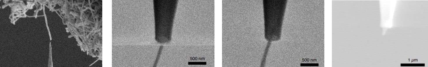
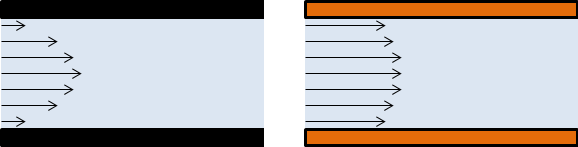
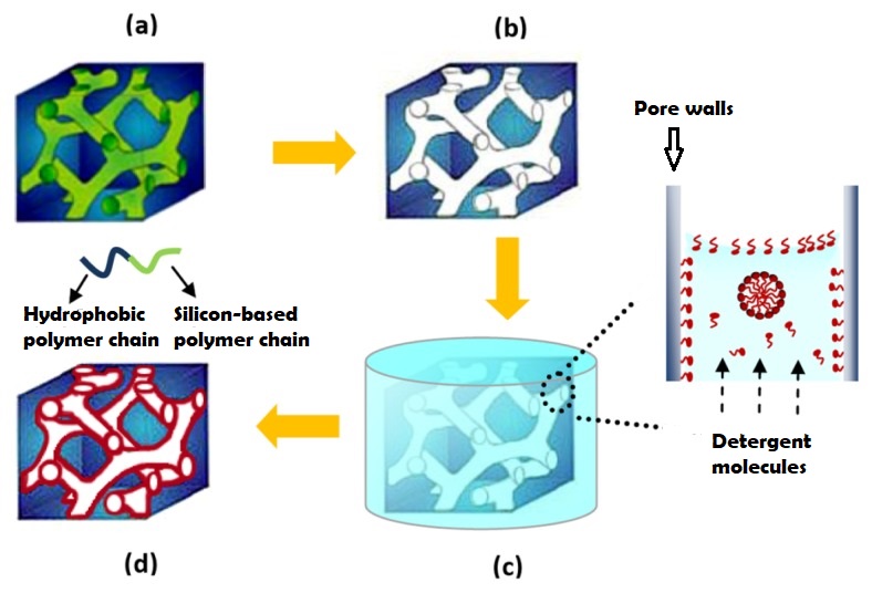
The nanoporous film used in this study is made of a polymer that has two hydrophobic (water-repelling) chains, one of which is a silicon-based material that we use in contact lenses. The polymer chains self-organize into the beautiful gyroid structure shown in Figure 2, which is a 3D interconnected surface that repeats in three directions (is triply periodic) and contains no straight lines. The most beneficial part of this structure is that it forms small, nanoscale pores after the removal of the silicon-based chains, which provide large storage space for the detergent molecules. To stabilize the final structure used in this study, the researchers add a chemical compound to remove the silicon-based chains. At this step, the interconnected polymer chains form strong covalent bonds with each other, a process called cross-linking. Figure 3 shows the process of the nanoporous film preparation (a, b) and loading of the detergent (c, d) (to learn more about the preparation, see [1]).
What happened to the E. coli communities after being in contact with the nanoporous film loaded with detergent? The researchers tested three samples of films differing in thickness (0.5mm, 1mm, and 1.5mm). They took microscopic images after two days and after seven days of contact with the bacteria. These specific periods were chosen because it is known that within three days almost 70% of the detergent can be released from the nanopores. To compare, they also included a nanoporous surface without detergent, which is shown in Figure 4, parts A and F. On the samples without detergent the bacteria were free to grow into large biofilms. The results in Figure 4 show the astonishing difference between the biofilms with, and without contact to the detergent after two days. Only a few small areas of live bacteria (green spots) were visible on the films with detergent, and even some dead bacteria were visible (red spots). The nanoporous surface worked! In addition, thicker nanoporous surfaces were even more effective against biofilm growth, because they have more pores loaded with detergent.
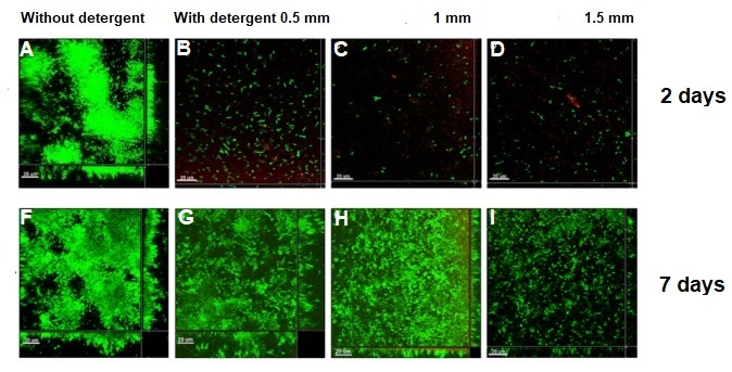
The tests after seven days were not as successful for the thinner films, which means most of the detergent was released from these films in less than seven days. Interestingly, the thickest nanoporous film was still effective at preventing biofilm growth after seven days. The researchers also tested the material on biofilms made by another type of bacteria, Staphylococcus epidermidis, which has a different type of cell wall. The results were not successful, and the biofilm kept growing, showing that the particular detergent is not effective in killing this type of bacteria. This shows the challenges researchers are facing, such as releasing antimicrobial compounds for longer periods of time and preventing the growth of specific bacterial species.
To conclude, this study showed that these gyroid nanoporous surfaces are effective in delivering detergent to prevent the formation and growth of E. coli biofilms. The researchers recommend further experiments with different types of detergents to target more species of bacteria. Of course, we can’t use detergents for applications in the body (detergents are highly toxic), but it is possible these nanoporous films could be used to deliver other non-toxic, antibacterial molecules. The research on the fight against biofilms keeps going! But you still have to visit your dentist every six months.
Continue reading “Anti-biofilm Material to Fight Bacterial Formation on Surfaces”