

Original paper: Fluid Dynamics of Bacterial Turbulence
The next time you’re washing your hands, start by turning the water on just a little. Notice how clear is the flow of the water from the tap. There aren’t any bubbles in the water, and when you put your finger in the stream, it smoothly flows around it. This is called laminar flow. Now keep increasing the water flow until it is very fast and rough. The chaotic nature of the flow in this stream is called turbulence, and how a flow turns from being laminar to turbulent is a popular area of research. In general, turbulent flows are very fast and are made from fluids that are not very thick.
In today’s study, Dunkel and his colleagues investigate how bacteria can make flow patterns that look turbulent – chaotic and full of vortices – even though bacteria are tiny and slow. The bacteria push the fluid around as they swim and create vortices, spinning regions in the fluid. The 5 ?m long bacteria create vortices with diameters of 80 ?m by swimming at the speed of 30 ?m/s!
To determine whether a fluid flow is turbulent or laminar, the Reynolds number, a ratio of the strength of the flow (inertial forces) to how much the fluid resists motion (viscous forces) is used and defined as [1]:
$latex Re = \frac{\rho V D}{\mu}$
It depends on the fluid density ?, flow speed V, the length of an object D (for example, the diameter of a bacterium), and flow viscosity, or thickness, ?. When the Reynolds number of a flow is high, the inertia of the fluid (how powerfully it flows), is much higher than its viscosity (how thick the fluid is). In this case, the resistance of the fluid to small fluctuations in its motion is not enough to prevent the fluctuations from growing and spreading. Before you know it, your previously smooth, easily predictable flow is chaotic and full of vortices – it has transitioned to turbulence.
Typically, flow in a pipe like that in a tap becomes turbulent at a Reynolds number of 2300; the flow of air over an airplane begins transitioning when the Reynolds number is about a million. Bacteria are so tiny and slow that their Reynolds number is very small – on the order of $latex 10^{-5}$.
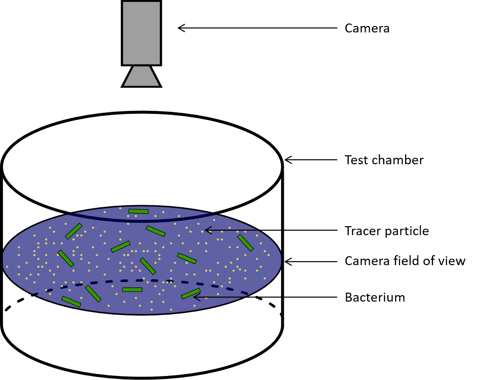
The researchers in this study investigate turbulent-like fluid behavior caused by swimming bacteria, B. Subtilis, in a fluid. B. Subtilis is a rod-like bacteria that swims by pushing its surrounding fluid with its flagellum (or tail). The researchers grew the bacteria in a nutritious fluid medium, and they added small, 1 micrometer beads to the fluid to act as tracer particles. When tracer particles are added to a fluid, you can see them being pushed around by its flow. If the particles are small enough, tracking them can be used to show how the fluid is moving. Thus, the experiment consisted of a suspension (a mixture in which particles do not dissolve) of bacteria and particles in the fluid.
The researchers loaded this suspension into sealed microfluidic cylindrical chambers with a 750 ?m radius and 80 ?m height (Figure 1). Since the chamber was sealed, the bacteria grew tired and did not move as much as they ran out of oxygen, so their activity levels decreased during the 10 minutes they spent in the chamber. Thus, by waiting several minutes between sets of measurements, the researchers were able to test how the bacteria affected the fluid at different energy levels.
The researchers took high-speed 2D videos of slices of the suspension containing the bacteria and the particles in the middle of the cylinder (even though the motion of the bacteria was in 3D). They used visible light to illuminate the motion of the bacteria and fluorescent light to view the motion of the tracer particles through a microscope.
.
The researchers used two methods to measure the motion of the suspension of bacteria and particles. First, by monitoring the motion of the bacteria, they obtained vectors showing how the bacteria were moving. Trajectories of bacterial movement were calculated by comparing the position pattern of the bacteria from one image frame to another. In the second approach, they tracked the motion of the particles in the flow by comparing the actual position of the particles from one image frame to the next. The researchers used both methods (monitoring patterns of bacterial motion and tracking individual particle positions) to make sure the flow fields measured from bacteria were an accurate representation of the flow. Since the tracer particles used by the researchers were very small, with diameters of 1 micrometer, they were small enough to be reliably pushed by the flow.
The typical results the researchers got are shown in Figure 2, with visible vortices.
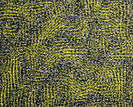
The researchers measured the velocity distributions of the bacteria. They found that the results from the tracer particles and the bacteria had the same distributions – the flow of the bacteria and solvent were very similar, and the flow of the bacteria could be used to represent the fluid flow. However, it is possible that the particles were pushed around by the bacteria, and not by the motion of the fluid itself, which is not mentioned in the paper.
To analyze the average motion of the bacteria, the researchers calculated various properties of the velocity field. They calculated the vorticity, $latex \omega_z$, or how much the bacteria rotated the fluid. The average of the square of the vorticity throughout the 2D experimental plane is called the enstrophy, $latex \Omega_z$. They then calculated the kinetic energy of the flow, $latex E_{xy}$, the energy a fluid has because of its speed, and also calculated its average throughout the space (1). Although the instantaneous kinetic energy and vorticity fluctuated as the bacteria moved, the average kinetic energy and enstrophy over time were approximately constant throughout the 50 seconds of recording.
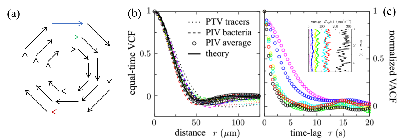
The researchers then measured two properties of the flow with functions called the VCF (“equal-time spatial velocity autocorrelation function”) and the VACF (“two-time velocity auto-correlation function”). The first function, the VCF, measures how the velocity of the fluid changes throughout the space (the 2D slice of the cylinder). If this function goes from positive, velocities in the same direction, to negative, velocities in different directions, then it indicates that there is a vortex in the fluid (Figure 3a). The results of the VCF are shown in Figure 3b. The researchers calculated that the radius of a vortex in the fluid was $latex R_v = 40 \mathrm{\mu m}$ from the VCF. The vortex radius did not change with the kinetic energy of the flow.
The average enstrophy was found to be linearly proportional to the time-averaged kinetic energy by about half the vortex radius ($latex \Lambda = \mathrm{24 \mu m}$) over all the energy scales tested:
$latex \overline{\Omega_z} =\frac{\overline{E_{xy}}}{\Lambda^2}$
So when bacteria have more energy, the fluid has a higher tendency to form vortices and rotate (but the vortices will be the same size).
The second property the researchers calculated was the “VACF”. The VACF measures how the velocity changes over time. The VACF represents the memory of the fluid. If it decays to 0 slowly, that means the velocities stay similar for a long time; if it decays quickly, the velocity changes in a very short time. The results of the VACF are shown in Figure 3c. The researchers found that at higher energies, the system has a shorter “memory”. The VACF shown in black has the highest energy, and decays much faster than the VACF shown in purple, which has the lowest energy. In bacterial turbulence, bacteria add energy to the system by swimming to make small vortices, which then lead to larger vortices. This is the opposite of how vortices form in a non-active turbulent fluid, where the energy is added to the larger vortices that create smaller vortices because of the fluid’s viscosity.
Finally, the researchers present a recently developed theory for the flow caused by bacteria. This theory is a continuum model equation – it treats the suspension of fluid, bacteria, and particles as if it were a continuous material, and accounts for the effects of the fluid flow and the forces the bacteria apply to the system.
The equation in the theory can be modeled to predict how the suspension will move. If the parameters of the equation in this theory are chosen to represent flow without bacteria, it simplifies to a theoretical fluid flow model. The researchers chose coefficients in the equation known to represent bacteria that push the fluid, like B. Subtilis in this experiment. They found that the model was accurate to within 10%-15%, making it a good candidate for a quantitative description of bacterial turbulence.
In today’s paper, Dunkel and his colleagues made significant contributions to the understanding of bacterial turbulence. The researchers developed a method to show that the motion of the bacteria swimming in a fluid can be used to measure the motion of the fluid itself. They developed a mathematical model of the motion and tested it with their experimental results to create a method for quantitatively studying how bacterial motion affects fluid flows. The observations they made can be used to compare bacterial turbulence to traditional turbulence in fluid mechanics, and give insight into how other fluids with active particles might behave.
[1] Fox, Robert W., Alan T. McDonald, and Philip J. Pritchard. Chapter 2, Introduction to fluid mechanics. Vol. 5., New York: John Wiley & Sons, 1998.
[2] Dunkel, Jörn, et al. “Fluid dynamics of bacterial turbulence.” Physical review letters 110.22 (2013): 228102.
(1) The vorticity, $latex \omega_z$, is calculated by taking the difference between the change in the y-component of the velocity, $latex v_y$, in the x-direction and the x-component of the velocity, $latex v_x$ in the y-direction:
$latex \omega_z = \frac{\partial v_y}{\partial x} – \frac{\partial v_x}{\partial y}$
The average kinetic energy (represented by angle brackets is calculated as:
$latex E_{xy} = \frac{v_x^2+v_y^2}{2}$
As the mass of the bacteria was constant, the energy depends only on the measured velocities of bacteria, and mass was not included in the calculation. As you may remember, a range of energies was tested by varying the bacterial activity.
The enstrophy, $latex \Omega_z$, is calculated as the average of the vorticity as:
$latex \Omega_z = \langle\frac{\omega_z^2}{2}\rangle$
2 Replies to “How swimming bacteria spin fluid”