Original paper: Mechanical stability of particle-stabilized droplets under micropipette aspiration
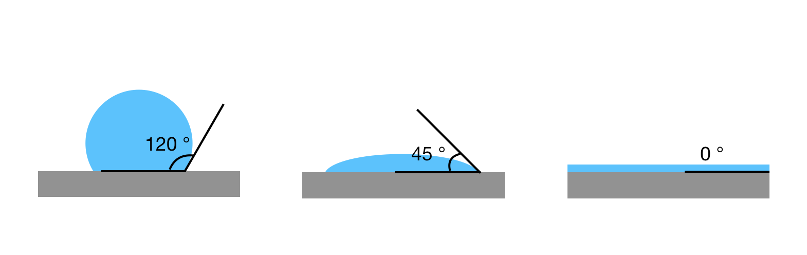
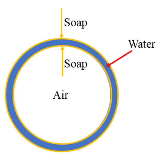
Most of us have had the childhood experience of blowing bubbles. But have you ever wondered how bubbles form and what keeps them stable? The key to making bubbles is surface tension, the tension on the surface of a liquid that comes from the attractive forces between the liquid molecules. Water has a very high surface tension (that’s why bugs can walk on water) making it difficult to stretch to form a thin water layer that we see when bubbles form. By adding soap to water, we can lower the surface tension of the water, allowing us to stretch this water-air interface to form a thin water sheet. As you blow more and more air into a bubble, the bubble will grow larger and larger as the thin layer stretches. Eventually, you’ll reach the limit of the added stretchiness, and the bubble will burst, engraving in your memory its fragile nature.
In soft matter, sometimes scientists utilize materials such as solid macroscopic particles instead of soap molecules to reduce the surface tension of an interface. Using particles to stabilize an interface allows them to tailor the mechanical and chemical properties of the interfaces to fabricate capsules. For instance, if a capsule needs to travel in blood-stream for therapeutic purposes, it must be tough enough to withstand blood pressure without rupturing. But if we make such a capsule how can we measure its mechanical response?
In this post, we’ll look into the work by Niveditha Samudrala and her colleagues on measuring the mechanical properties of a particle-stabilized interface. They utilize a direct approach of applying force on such a stabilized interface to study its mechanical response that has eluded earlier techniques. Knowing the stiffness of these particle-coated interfaces, say in the form of capsules, would enable us to use them for different controlled-release applications such as treating a narrowing artery [1] as well as tune them to have different flow properties.
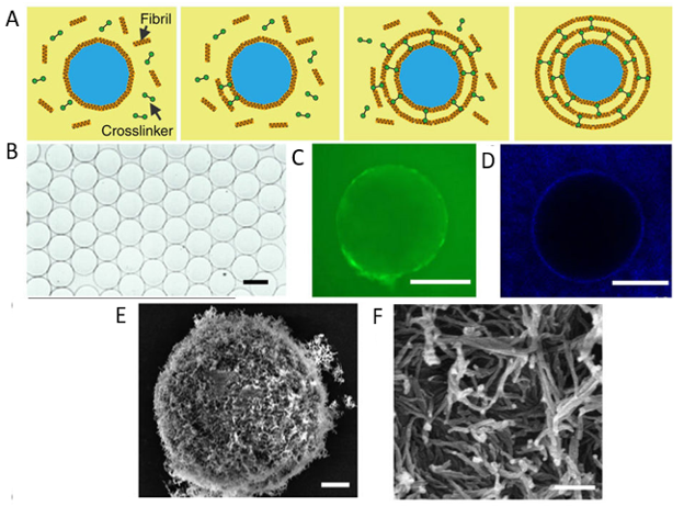
The authors use tiny (smaller than a micrometer!) dumbbell-shaped particles with different surface properties to stabilize an oil-in-water emulsion (see note [2]). Here instead of a thin layer of water sandwiched by the soap molecules, the water-oil interface has been stabilized with micron-sized particles. This stabilization technique will render higher mechanical properties to the interface. Droplets stabilized in this way, known as colloidosomes, have been shown to be capable of encapsulating a wide variety of molecules.
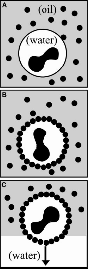
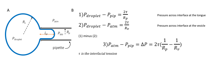
The researchers characterized the particle-stabilized droplets using the micropipette aspiration technique. To understand this technique, imagine picking an air bubble with a straw. What you need to do is to approach the air bubble and then apply a gentle suction (or aspiration) pressure. When the suction pressure becomes larger than the pressure outside of the droplet, then the droplet gets aspirated into the straw forming the aspiration tongue (Figure 1A). Similarly, in the micropipette aspiration technique, a glass pipette (the straw) with an inner diameter of $latex R_p$ is usually used to aspirate squishy stuff, such as cells, vesicles, and here droplets.
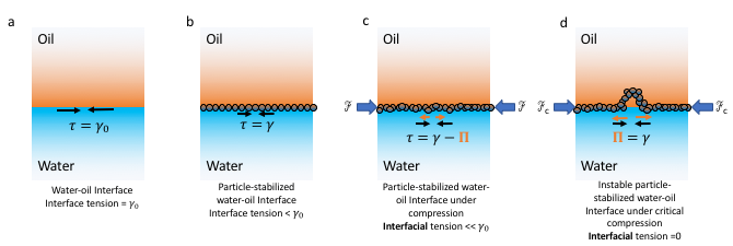
To obtain the tension response, therefore the toughness of an aspirated interface, we need to consider the pressures applied to the interface. Let’s consider an aspirated droplet as shown in Fig 1A at mechanical equilibrium (which means the sum of all the forces is zero). We know that each interface has a surface tension acting on it (See Fig 2a). In our bubble example, I mentioned that the soap molecules tend to gather at such interface to decrease the tension (See Fig 2b). But when there are other forces acting on the interface in addition to the presence of the molecules, such as the suction pressure in our case, the tension of the interface now comes from both the surface tension and the suction force. We call this total force the interfacial tension (See Fig 2c). The Young-Laplace equation can be used to relate this interfacial tension to the pressure applied to the interface (Fig 1-B3).
When the molecules, or particles in our case, are forced to pack tightly together they oppose the compression force. This opposition is felt at the interface by a pressure called surface pressure (see Fig 2c). Under the interface tension and the surface pressure, the new net interfacial tension is defined as:
$latex \tau=\gamma_{0} – \Pi$.
where $latex \Pi$ is the surface pressure, $latex \gamma_{0}$ is the interface tension which is constant for a given interface.
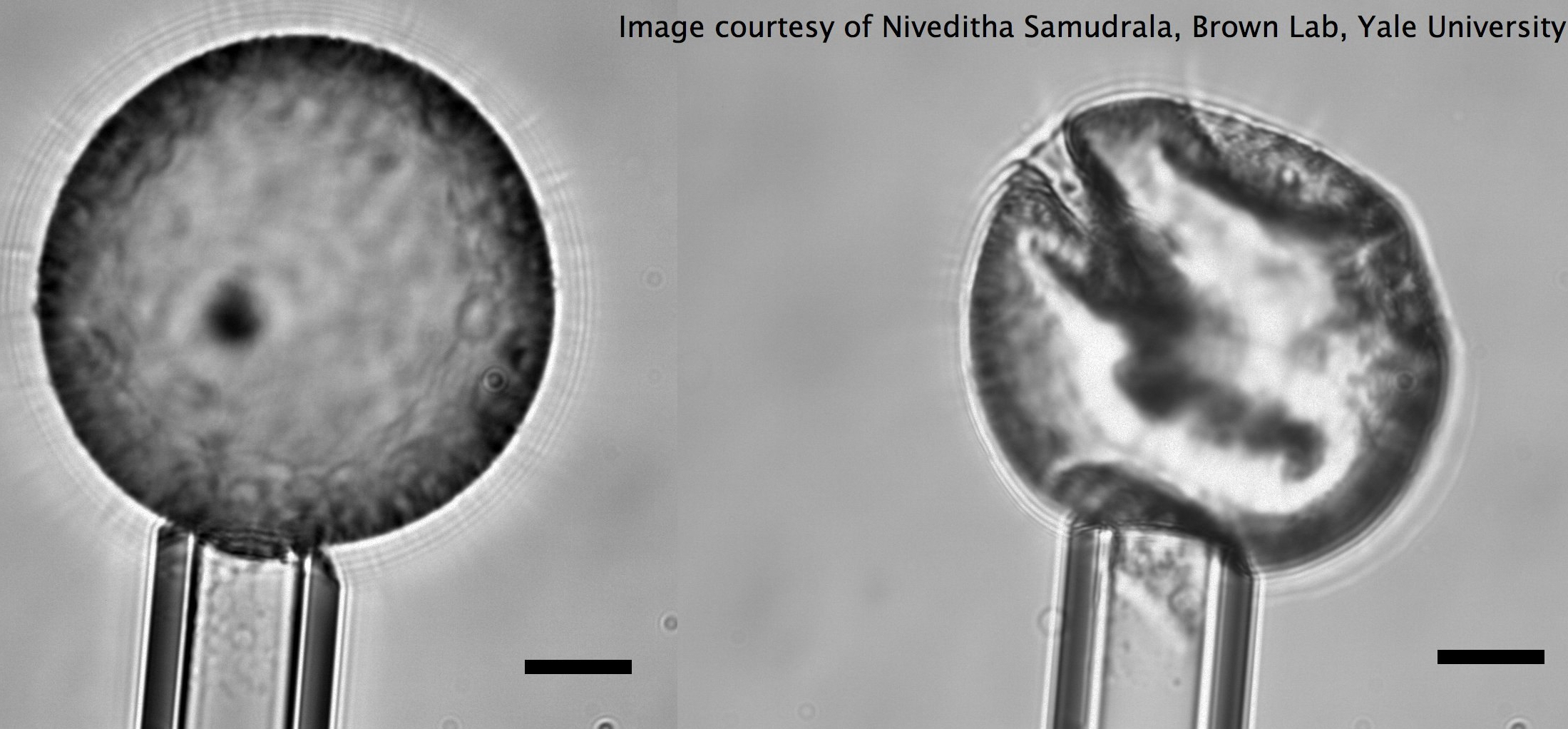
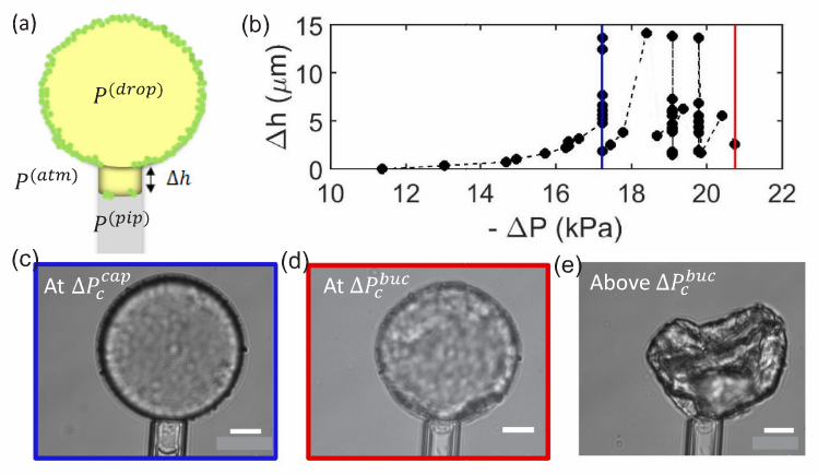
In this study, Samudrala and her colleagues show that there are two critical pressures after which instabilities form at the interface resulting in droplet dripping into the pipette and buckling respectively (Fig 2d). They conclude that the dripping happens due to the transition of the interface from a particle-stabilized interface to a bare oil-water interface resulting in a sudden suction of tiny oil droplets (basically the droplet drips at this point, see Fig 3B, blue and 3C).
The second instability is the buckling which the researchers propose happens when $latex \tau$ tends to zero. Now let’s see how buckling happens.
The dripping at the first critical pressure decreases the volume of the particle-coated droplet, but note that the surface area is constant because neither particles leave the surface nor the free ones join the droplet (the latter argument is assumed). The continuation of the increase in suction pressure plus the volume lost in the dripping step results in the buckling of the interface (Fig 3b red and 3E, also see note [3]). When the authors aspirate the bare oil droplets as well as droplets stabilized by small molecules, they only see the sudden droplet disappearance with no shape abnormalities due to the fluid nature of the interface rather than solid-like nature for the particle-stabilized case. But why does the buckling happen?
Recall how we defined the net interfacial tension above; $latex \tau=\gamma – \Pi$. The authors hypothesize that upon suction of a particle-stabilized droplet, particles jam at the interface of the droplet outside of the pipette, creating a high surface pressure. When this surface pressure approaches $latex \gamma$, the net tension becomes zero ($latex \tau=0$, see fig 2d and note how the interface tension is opposed by the surface pressure due to repulsion between particles). When an interface possesses no tension, it means that the interface can no longer bear any loads. Considering any sort of defects or irregularities due to nonuniform particle packing, for such interfaces deformations such as buckling will form. Now, let’s see how the authors test their hypothesis.
The authors observed that at the tip of the tongue, there is a very dilute packing of particles in such a way that the interface to a good approximation resembles the Fig 2a, a bare water-oil interface. With this observation, one can safely assume that the interfacial tension, the $latex \tau$ is equal to the oil/water interface tension, the $latex \gamma$ and write the Young-Laplace equation across the tip of the tongue (see Fig 1B-(1)):
$latex P_{droplet} – P_{pip} = \frac{2\gamma_{0}}{R_{p}}$
where $latex R_{p}$ is the radius of the pipette and is fixed. The authors experimentally show that for a range of droplet size ($latex 10\ \mu m < R_{droplet} < 100 \ \mu m$), the droplet pressure right before buckling varies very close to zero (in above equation all parameters are known except the $latex P_{droplet}$, which is calculated when we put $latex P_{pip} = P_{buckling}$). Therefore, considering the equation (2) in Fig 1B, the net tension would be zero (see note [3]) and with this, the authors correlate that the reason for the formation of buckling is the net-zero tension of the interface.
Taking it all together, we saw that for a droplet with solid-like thin shell, the mechanical response is completely different from the bare or the molecule-stabilized interface. A fairly rigid interface undergoes buckling due to its net tension tending to zero and knowing the threshold of buckling will enable us to tune the mechanical properties of such droplets for different applications from load-caused cargo release (see note [1]) or emulsions with varied flow properties. Imagine if we encapsulate a fragrance in our air bubble, which upon rupturing will release the scent. Now, wouldn’t it be nice if we could control the toughness of this bubble or similar architecture to rupture under a specific condition that we desire (see note [1])?
[1] In a disease called atherosclerosis, the arteries narrow down due to plaque buildup. In this narrow region, the blood pressure is higher than the normal region of the artery. So one can use this pressure difference to crack release the relevant drug from the capsule only in the narrow regions of the artery to dissolve the plaques away. Neat!
[2] If we apply a shear force on a mixture of two or more immiscible liquids in the presence of a stabilizing agent, we produce an emulsion and the stabilizing agent is called an emulsifier. The particles show a significantly higher tendency to gather at an interface in comparison to amphiphilic molecules. Thus, particles are strong emulsifiers. If we mix lemon juice and oil, soon after stopping the mixing, the two solutions will separate. Now, if you add eggs, you stabilize this mixture (egg works as an emulsifier) and you get Mayonnaise!!
[3] The authors report that for particle-stabilized droplets they observed different deformation morphologies such as wrinkles, dimples, folds and in some case complete droplet failure. They attribute this diversity to the non-uniformity of particle packing at the interface. But what is interesting to me is when they decrease the suction pressure, the droplets go back to their original spherical shape and then upon the second aspiration, the deformations happen at the same exact location as were for the first aspiration. This means that during the suction, there is limited particle rearrangement (Watch here).
[4] We can easily set the atmosphere pressure to zero before aspirating the droplets, thus here the $latex P_{atm} = 0$.