Original paper
A General Model for the Origin of Allometric Scaling Laws in Biology. By Geoffrey B. West, James H. Brown, and Brian J. Enquist. Science 1997
Physics is a discipline that attempts to develop a unifying, mathematical framework for understanding diverse phenomena. It connects things as different as planets orbiting the sun and a ball thrown through the air by showing that both these motions come from a single equation [1]. Living things do not seem to obey such simplicity, but hidden beneath all the diversity and complexity of life are remarkably universal patterns called scaling laws. In a landmark 1997 paper by Geoffrey West, James Brown, and Brian Enquist, a simple explanation is given for how all organisms, from fleas to whales to trees, can be thought of as non-linearly scaled versions of each other.
A scaling law tells you how a property of an object, say the rate at which energy is consumed by an organism (its metabolic rate), changes with the object’s size. Just by looking at the data, many quantities scale as a power law of the mass,
$latex A \propto M^{\alpha}$ (Eq. 1)
where ? is some number that, from the data, always seems to be a multiple of 1/4 [2]. West, Brown, and Enquist build a theory showing how biology could have come up with this 1/4 power law, but in this article, I’m just going to focus on one specific example. I’m going to walk through the author’s arguments for how the metabolic rate, the rate at which an organism consumes energy, scales with an exponent of 3/4. They show that it all comes up from some basic assumptions about the networks that distribute nutrients to your body — your circulatory system [3].
These networks are assumed to have two characteristics [4]. First, they are space-filling fractals. Fractals are shapes made of smaller, repeating versions of themselves no matter how far you zoom into it. However, our fractal blood vessels can’t get arbitrarily small, they have a “terminal unit”— the capillary. The second assumption about these networks is that all terminal units are the same size, regardless of organism size. With these two assumptions, the authors are able to derive the 3/4 power law for metabolic rate.
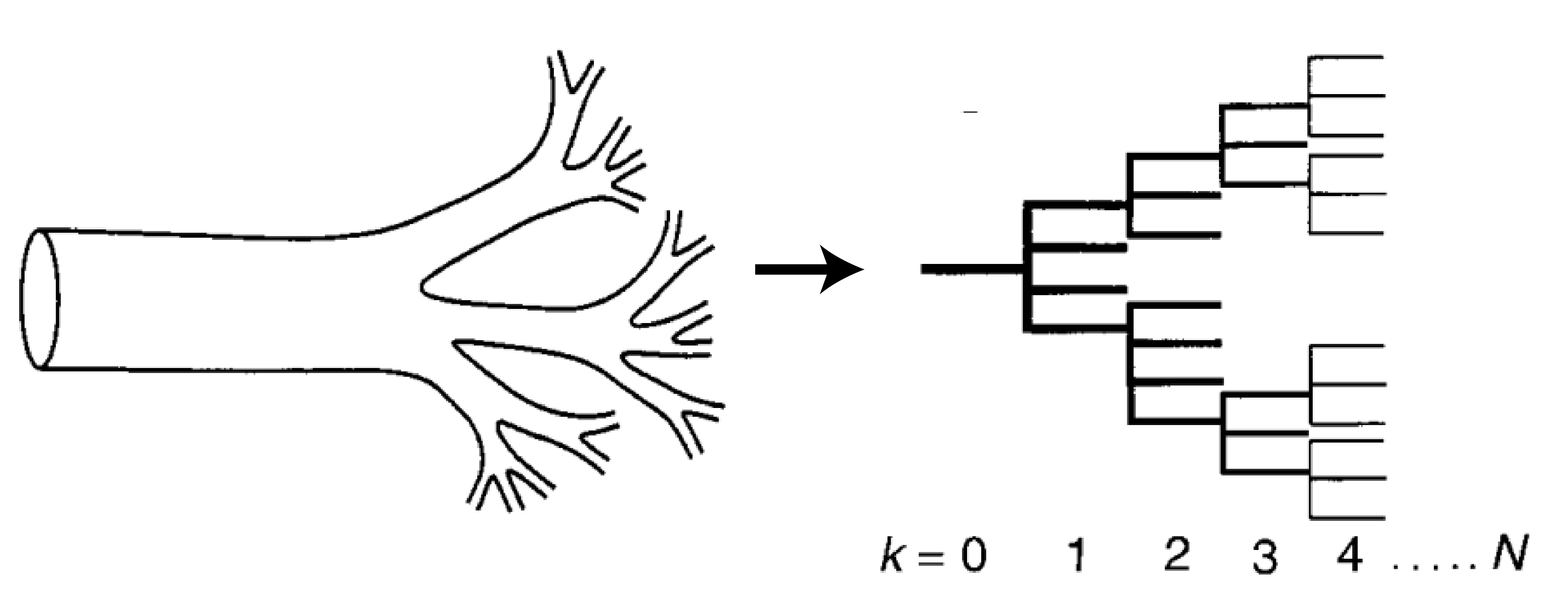
First, let’s build up a picture of what these networks look like. Figure 1 shows how the circulatory system can be thought of as a network structured into N levels, where each level k has $latex N_k$ tubes. At each level, a tube breaks into a number ($latex m_k$) of smaller tubes. Each one of these tubes is idealized as a perfect cylinder with length $latex l_k$ and radius $latex r_k$, as shown in Figure 2.
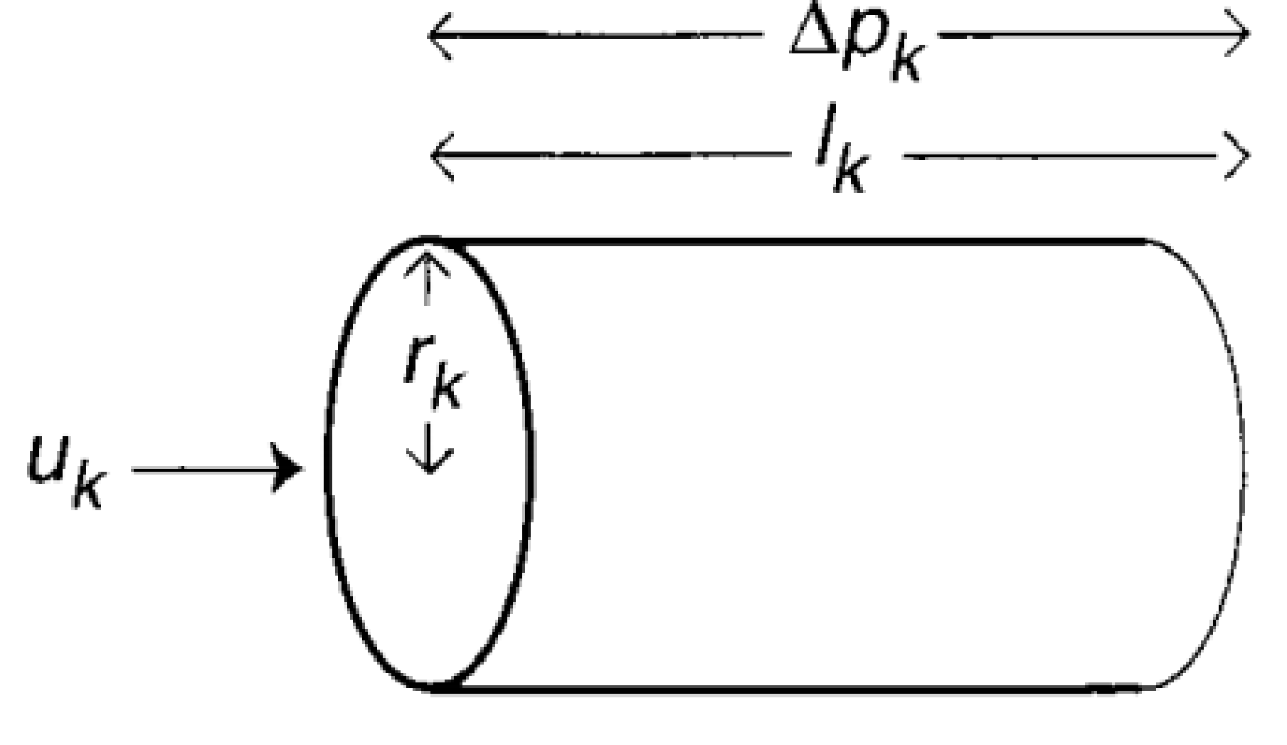
How does blood move through this network? Well, the blood flow rate at each level of the network must be equal to the blood flow rate at every other level. Otherwise, you would have the equivalent of traffic jams in your arteries. You don’t want those. If the blood flow speed through one tube in the kth level is $latex u_k$, the blood flow rate through the entire kth level is
$latex \dot{Q}_k = N_k \pi r_k^2 u_k = N_{cap} \pi r_{cap}^2 u_{cap} = \dot{Q}_{cap}$ (Eq. 2)
Your metabolic rate, B, depends on the flow rate through your capillaries, $latex \dot{Q}_{cap}$, so the authors assume that the two are proportional to each other: $latex B \propto \dot{Q}_{cap}$. Because all terminal units are the same size, the only variable left in Eq. 2 to relate to an animal’s mass is $latex N_{cap}$. Assuming that B scales like $latex B \propto M^{\alpha}$, and the authors predict
$latex N_{cap} \propto M^{\alpha}$ (Eq. 3)
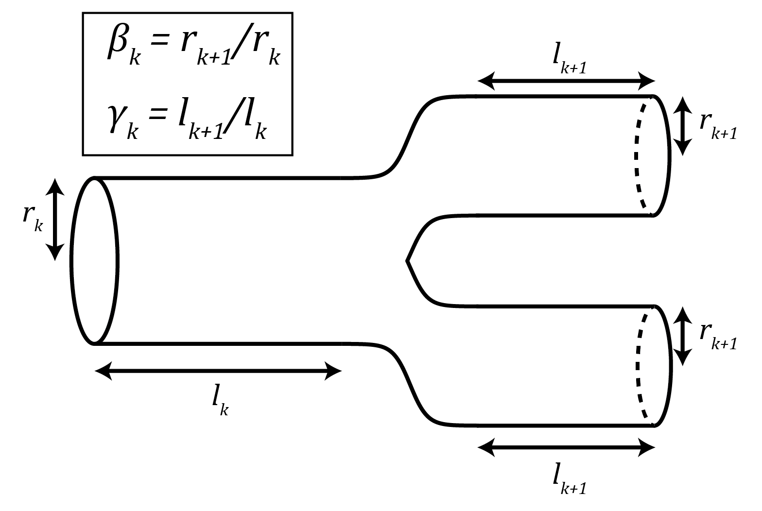
To figure out the value of the exponent $latex \alpha$, the key is to get $latex N_{cap}$, which depends on the size of the organism, in terms of the capillary dimensions $latex r_c$ and $latex l_c$, which do not. To do this, the authors use relations derived using the self-similar geometry of the fractal network. When a tube breaks into smaller tubes, it does so with a ratio between the successive radii, $latex \beta_k = r_{k+1} / r_k$, and another ratio between the successive lengths, $latex \gamma_k = l_{k+1}/l_k$. This is illustrated in Figure 3. Because the network is fractal, the number of tubes each branch breaks into, $latex m_k$, the ratio of radii, $latex \beta_k$, and the ratio of lengths, $latex \gamma_k$, are all assumed to be constant for every k,
$latex \beta_k = \beta, \; \gamma_k = \gamma, \; m_k = m \;\; \forall k$
Since, at every level, each branch breaks into m smaller branches, the total number of capillaries (i.e. the number of branches at level N) is $latex m^N$. Plugging this into Eq. 3,
$latex \alpha = \frac{N \ln(m)}{\ln(M/M_0)}$ (Eq. 4)
Where $latex M_0^{\alpha}$ is the proportionality constant between $latex N_{cap}$ and $latex M^{\alpha}$. Remember, we’re trying to show that $latex \alpha = 3/4$.
Now that $latex N_{cap}$ has been rewritten in terms of network properties, the authors next turn their attention to another quantity that scales with the organism size — its mass, M. To do this, the authors use the empirical fact that the total volume of blood, $latex V_b$, is proportional to the total mass of the organism, $latex V_b \propto M$. The total volume of blood is given by:
$latex V_b = \sum_{k=0}^N V_k N_k = \sum_{k=0}^N \pi r_k^2 l_k m^k \propto \left( \gamma \beta^2 \right)^{-N} \propto M$ (Eq. 5)
In the above equation, the first proportionality sign (summing the series) requires a calculation that’s given here. The main idea of this calculation is that, because the ratios $latex r_{k+1} / r_k$ and $latex l_{k+1}/l_k$ are each constant, the sum in Eq. 5 can be turned into a geometric series which can be summed analytically. Plugging the final proportionality from Eq. 5 into Eq. 4,
$latex \alpha = – \frac{\ln(m)}{\ln(\gamma \beta^2)}$ (Eq. 6)
To make further progress, we have to know something about $latex \gamma$ and $latex \beta$. Every tube of the network gives nutrients to a group of cells. As every good physicist does, the authors will assume that this group of cells has the volume of a sphere with a diameter equal to the length of the tube. The volumes serviced by each successive level are approximately equal to each other, $latex 4/3 \pi (l_{k+1} / 2)^3 N_{k+1} \approx 4/3 \pi (l_k / 2)^3 N_k$. From this, they get an expression for $latex \gamma$:
$latex \gamma_k^3 \equiv \left(\frac{l_{k+1}}{l_k}\right)^3 \approx \frac{N_k}{N_{k+1}} = \frac{1}{m}$ (Eq. 7)
which means
$latex \gamma \approx m^{-1/3}$
Now the authors move on to $latex \beta$. Earlier, I argued that the flow rate has to be the same from one level of the network to the next to avoid “traffic jams” of blood. Since the tubes are assumed to be perfect cylinders, this boils down to the idea that the cross-sectional area of a parent tube being equal to the total cross-sectional area of its daughter tubes, $latex \pi r_k^2 = \pi r_{k+1}^2 m$. From this, the authors find an expression for $latex \beta$:
$latex \beta_k^2 \equiv \left( \frac{r_{k+1}}{r_k} \right)^2 = \frac{1}{m}$ (Eq. 8)
Similar to the expression for $latex \gamma$, this means
$latex \beta \approx m^{-1/2}$
Plugging in the expressions for $latex \gamma$ and $latex \beta$ in terms of m, we finally arrive at our desired result:
$latex \alpha = – \frac{\ln(m)}{\ln(\gamma \beta^2)} = – \frac{\ln(m)}{\ln(m^{-1/3}(m^{-1/2})^2)} = 3/4$ (Eq. 9)
What West and his colleagues have done is use the fact that all organisms have to deliver nutrients to their individual parts to derive a general, universal scaling law. The authors go on to show that when you add a pump to the system, such as our heart, the analysis may get more complicated, but the ultimate result remains unchanged. All living things, regardless of size, seem to have arrived at the same solution for nutrient supply, building systems that are space-filling, fractal, and have the same size “terminal units”. Turns out we’re not so different after all.
[1] $latex F = Gm_1 m_2 / r^2$. ^
[2] For example:
- $latex \alpha = 3/4$ for cross section area of aortas of mammals, tree trunk sizes
- $latex \alpha = -1/4$ for cellular metabolic rate, heartbeat rate, population growth
- $latex \alpha = 1/4$ for time of blood circulation, life span, embryonic growth rate ^
[3] All the arguments hold for other distribution systems, such as our pulmonary system, plant vascular systems, and insect respiratory systems. ^
[4] There’s an additional assumption that the network is designed to minimize energy, but that won’t come into play in the part of the author’s arguments that I will be presenting here. ^