Many consumer products, such as clothes and food packaging, are made of blends of polymers, long molecules consisting of repeating chemical units. The attractiveness of using blends of different polymers arises from the engineers’ desire to combine multiple unique properties of each individual polymer, such as transparency, stretchability, and breathability, into a seamless whole. However, different polymers are not necessarily miscible, a term scientists use to describe whether two materials mix at the molecular level. Miscibility isn’t a one-and-done kind of deal: scientists and engineers have known for years how to make polymer blends mix by careful temperature control. What if there were conditions other than temperature to achieve polymer blend miscibility? This may ultimately help in industrial processing of polymer blends. In this week’s paper, Professors Annika Kriisa and Connie B. Roth from Emory University in Atlanta, Georgia, explore the mixing dynamics of two polymers by using a strong electric field.
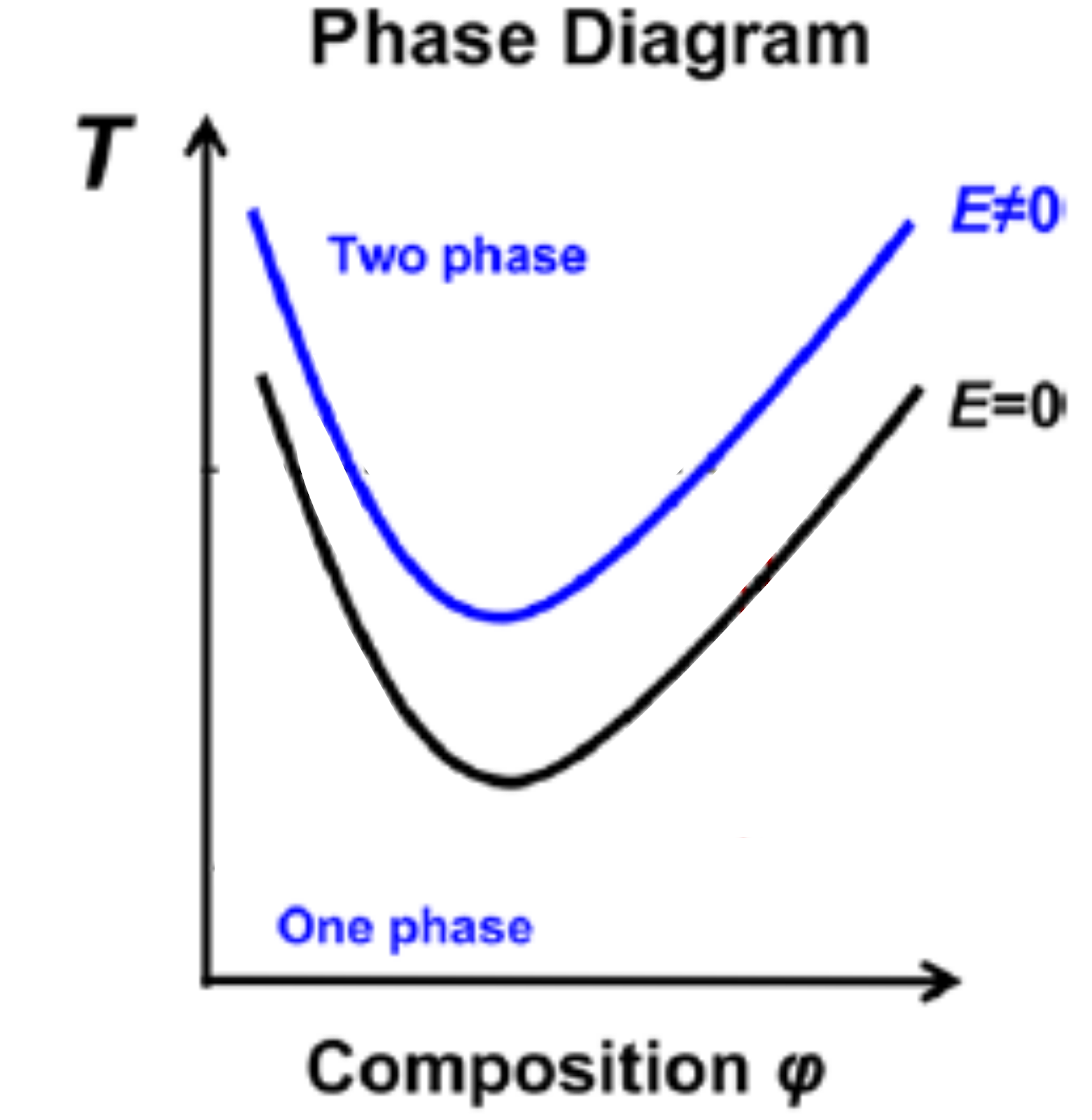
Figure 1. Miscibility diagram of a hypothetical polymer blend consisting of polymers A and B. The x-axis is the fraction of polymer A in the blend (Composition ?) and the y-axis is the temperature of the blend (T). The curves represent the temperature above which the blends are immiscible without an electric field (black curve) and with an applied electric field (blue curve). The presence of the electric field increases the miscibility of the blend (higher transition temperature) at a given fraction of polymer A. (Image adapted from original paper.)
Before we dive into the meat of the paper, it’s important to know how temperature affects the miscibility of a polymer blend. The black curve in Figure 1 is a representative miscibility diagram of two blended polymers, which shows the temperature at which a polymer blend transitions from being miscible (below the black curve) to immiscible (above the black curve) as a function of the fraction of one polymer (denoted Composition ?) of the blend itself. The polymer blend is considered more miscible if the miscibility curve is shifted upwards, so that the blend turns immiscible at a higher temperature (see blue curve in Figure 1).
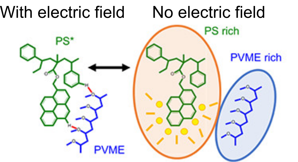
Kriisa and Roth wanted to explore how the application of an electric field influences the mixing dynamics of polystyrene (PS) and poly(vinyl methyl ether) (PVME) polymers. You may be quite familiar with these materials: PS is the formal name of styrofoam, the main component in plastic cups, and PVME is typically used in glues and adhesives. In the past, Kriisa and Roth studied the effect of electric fields in blends of these materials, and found that the electric field enhances polymer blend miscibility: an electric field raises the temperature at which a PS/PVME blend becomes immiscible, similarly to the blue curve in Figure 1 [1]. What interested the authors the most in this today’s paper was the dynamics of mixing; in other words, how quickly do immiscible blends remix once they are exposed to an electric field? And what can we learn about the factors governing the remixing process?
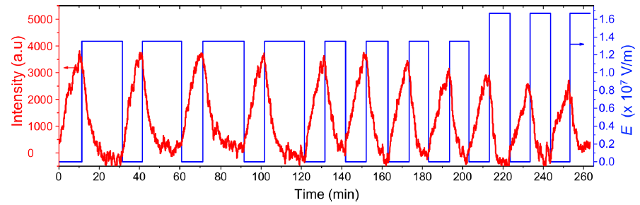
Figure 2. Switching the miscibility of polystyrene/polyvinyl ethyl ether (PS/PVME) polymer blends as a function of time through the application of an electric field (E). The red curve is the intensity of the fluorescence of a molecule attached to polystyrene, which decreases with time. The blue curve is the imposed electric field, which is repeatedly switched on and off. (Image adapted from original paper.)
The authors showed that the dynamics of mixing a PS/PVME blend is highly sensitive to the application of an electric field. They demonstrated this by examining a PS/PVME blend at the temperature four Kelvin higher than the temperature at which it becomes immiscible. They repeatedly switched on and off an electric field regularly, causing the blend to switch from being miscible to immiscible (see blue curve in Figure 2). To determine how well mixed the blend was, they measured the intensity of the light emitted by a fluorescing molecule, which was chemically attached to the PS molecules (see red curve in Figure 2). When PS and PVME are fully mixed, the fluorescence intensity decreases to 0. After switching on the electric field, the blend starts mixing immediately, showing a high sensitivity to the presence of the electric field.
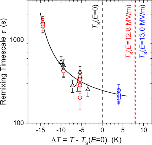
Figure 3. Remixing timescale (?) as a function of temperature (T) and applied electric field (E). The black symbols correspond to absence of electric field, red to electric field at E =12.8 MV/m, and blue at E=13.0 MV/m. Ts (shown by the dashed lines) is the temperature at which the blend becomes immiscible at the given electric field. The remixing timescales follow the same black curve, showing that they are largely independent of E. (Adapted from original paper.)
The authors repeated this experiment for a variety of temperatures and electric field strengths. From the fluorescence curves, they extracted the remixing timescale or the time it takes for the blend to remix, as shown in Figure 3. The black symbols correspond to absence of electric field, while the red correspond to E = 12.8 MV/m and the blue to 13.0 MV/m. One may notice that the time it takes for the polymer blend to remix is largely independent of the electric field strength at a given temperature, since all remixing timescales (?) follow the same black curve. Thus, the authors concluded that the rate of remixing is not affected by the electric field.
In short, Kriisa and Roth showed that the dynamics of remixing polymer blends are sensitive to electricity. They found that immiscible blends immediately begin to remix when exposed to an electric field and that the time it takes for the blend to completely remix is independent of the field’s strength. From an industrial perspective, this shows that the miscibility of polymer blends can be influenced by factors other than temperature. An important advantage is that an electric field can be applied uniformly and instantaneously, whereas changes in temperature take time to propagate through materials. Thus, engineers may be able to instantly tune the miscibility of polymer blends using electric fields; a discovery that may lead to future technological advances in devices and materials whose properties would be quickly ‘’switched’’ through electricity.
When an experiment doesn’t behave the way we expect, either our understanding of the relevant physics is flawed, or the phenomenon is more complicated than it appears. When a theoretical prediction is off by two orders of magnitude – like what was observed in this recent paper by Hua Yung Lo, Yuan Liu, and Lei Xu of the Chinese University of Hong Kong – something is seriously wrong.
If Lo and colleagues drop a liquid droplet onto a smooth, flat surface, it will take on an equilibrium shape which depends on the properties of the liquid and solid materials at the interface (eg. water on Teflon will form a nearly perfect spherical drop while water on stainless steel will spread out, forming a spherical cap). For low viscosity fluids, the equilibration process happens almost instantly… unless the surface is very flat and very smooth.
If the surface below a droplet is atomically smooth (not a single atom is out of place to roughen the surface), a thin layer of air will form between the droplet and the surface, keeping the droplet from making contact with the surface. Eventually the trapped air will escape, draining out like how a liquid would, allowing the droplet to collapse onto the surface. Traditional fluid dynamics simulations predict that the collapse would take between 10 – 100 seconds. In experiments, however, contact generally happens in less than one second. Lo and coworkers set about investigating this seeming contradiction by observing the flow that happens within the air and liquid at the boundary between a droplet and a smooth surface.
To study this problem, the researchers dropped small spherical oil droplets (1.7 mm diameter) onto a glass surface with a very thin coating of oil which could be tilted. They observed that droplets would compress and bounce as they floated on a pocket of air, before collapsing onto the surface. The contact area was imaged from the bottom and side simultaneously using two high-speed cameras. Side-on sequences are shown in Figure 1 with a slightly tilted surface (a) and a perfectly leveled surface (b). While both droplets collapsed onto the surface far quicker than predicted by simulations, the droplet on the leveled surface was observed to float just above the surface approximately 10 times longer than on the tilted surface before collapsing.
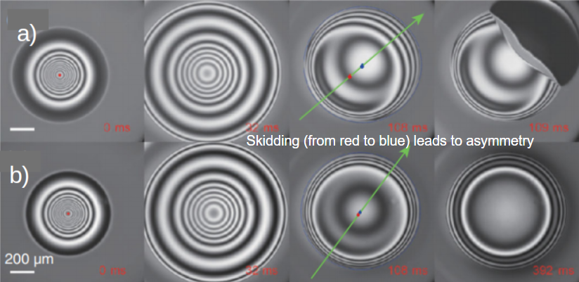
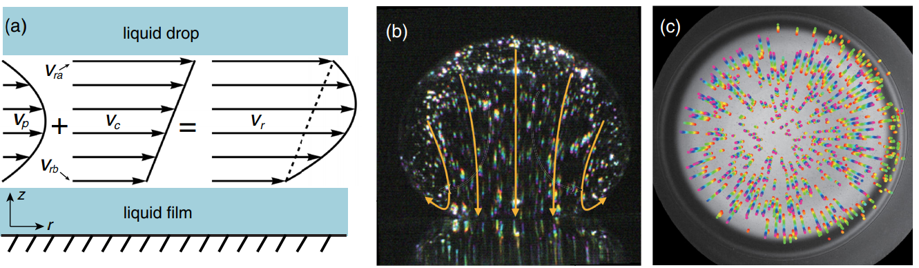
Figure 1. A time sequence of an oil droplet being dropped on an atomically smooth, oil coated, glass surface which is a) slightly tilted (0.3°) and b) leveled (0°). c). Schematic of the droplet and surface. A video of the process can be found here (Figure adapted from the original paper.)
The effect the tilted surface has on this phenomenon became more apparent when viewed from below. On the tilted surface, the droplet would “skid”, observed as a sliding of the droplet’s center from the red point to the blue point in the direction of the green arrow as shown in Figure 2 a) while the size and shape of the air pocket was measured using two-wavelength interferometry [1]. Tilting the surface caused an asymmetric air pocket to develop, with a thinner gap at the front of the droplet and a thicker gap at the back. When a droplet did not skid, it formed a symmetric air pocket like in Figure 2 b). A thinner gap (with difference of just half micrometer) lets the air drain out (and allows contact to be made) much faster than it would for a symmetric air pocket on a flat surface. However, even a flat surface drained 10-times faster than expected.
Figure 2. Images of the bottom of an oil droplet coming in contact with an oil-coated glass slide that is a) slightly tilted, showing a droplet skidding until it reaches full contact with the surface at 109 ms, and b) perfectly leveled, where the droplet still has not contacted the surface at 392 ms. Light and dark bands correspond to the change in thickness of the air pocket. A video of the process in a) and b) can be found here and here.
To understand the flow of air from under the droplet, the researchers modeled it as a low-viscosity fluid. When a low-viscosity fluid flows past a wall (like water through a tube), the friction at the walls may reduce the flow near the walls to something-close-to-zero. This is called a “no-slip boundary condition”. On the other hand, a “plug flow boundary condition” means there is significant slip and therefore flow along the walls. Each of these boundary conditions lead to characteristic velocity profiles like those presented in Figure 3 a). Typically, one would assume that air flowing through the air pocket near the oil interface would have a no-slip boundary condition while something like a sludge or gel would demonstrate plug flow. Yet, it is this assumption that ends up being incorrect.
The researchers measured the velocity of oil within the oil droplet and the surface coating using particle image velocimetry, a technique where small light-reflecting particles are mixed into a material and tracked down as they move along with the surrounding fluid. An image of the oil droplet seeded with the tracer particles is shown in Figure 3. In this way, the researchers were able to directly visualize flow of oil at the air-oil boundaries, finding a sort of “slip layer” along the walls corresponding to the layer of oil being dragged along by the air. This lets larger volumes of air drain from under the droplet, explaining the surprisingly short time it takes for droplets to collapse onto the surface.
Figure 3. a) The velocity profile of air under the droplet (Vr) is a combination of a no-slip (Vp), and slip (Vc) boundary conditions. b) Side-view image of an oil droplet. White dots are reflective particles with velocity shown as yellow arrows. c) Bottom-view of the same oil droplet where the colored streaks (red to purple) trace the flow of the oil on the surface. (Figure adapted from the original paper.)
Despite its apparent simplicity, Lo et al. revealed a fundamental misunderstanding in the way scientists thought about how fluids flow near an interface. Accounting for the effect of slip, the researchers unified both theory and observation and explain why liquid droplets will make contact with a perfectly smooth surface so much faster than originally expected.
[1] a technique that uses light interference to quantify changes in thickness as light and dark bands; narrow bands correspond to rapidly changing thicknesses, much like the lines on a topographic map show changes in elevation. ^
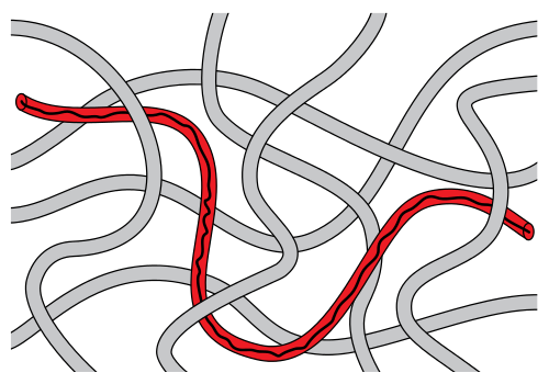
Scientists often draw inspiration from biological organisms to describe phenomena, even when they are studying outside the realm of biology. Physicist Pierre-Gilles de Gennes[1] was no exception. In 1971, after being inspired by the movement of snakes, he proposed reptation theory, or the reptation model, which has since been widely used to describe motions of polymers[2]. As the name “reptation” suggests, de Gennes assumed polymer chains move like snakes. As shown in Figure 1, the model describes a polymer chain’s motion in an environment that is highly populated by other chains (shown in gray) by assuming that the chain is confined in a virtual tube (shown in red) formed by surrounding polymer chains. According to reptation theory, the chain wiggles through this tube, similar to a snake slithering through the woods. As one might imagine, directly imaging the snake-like slithering of polymers is a challenging affair; however, in today’s study, Maram Abadi and coworkers from King Abdullah University of Science and Technology were able to do just that with DNA chains – an example of a polymer – and compared their results to prevailing theory.
Figure 1. A schematic of the reptation model. In a crowded and entangled polymer environment, a long and linear polymer chain (black) is located in a virtual tube (red), which traces the chain trajectory. Surrounding polymers are shown in gray. (Adapted from the Wikipedia page for reptation.)
While reptation theory has done fairly well in describing experimental observations of polymers, there are some shortcomings to both the experiments supporting this theory as well as to the theory itself. Namely, previous experiments mostly considered the overall motion of the chain; but local chain motion, such as motion at the ends of a polymer chain, have not been thoroughly studied. In addition, the theory was only designed for polymers with two ends, known as linear polymers. Thus, it does not account for the dynamics of polymers with different geometries, such as those that form rings, known as cyclic polymers. Given these observations, Abadi and coworkers realized that there was more work to be done in the studies of polymer dynamics.
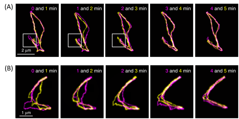
To scrutinize the movements of the polymer chains, the authors used super-resolution fluorescence localization microscopy[3], which lets them monitor the movements beyond the typical microscopy resolution of ~200 nm. This technique allowed Abadi and coworkers to not only observe whole-chain dynamics but also local dynamics. To test the predictions of reptation theory, they chose both linear and cyclic DNAs with fluorescent dyes attached as model polymers for their study.
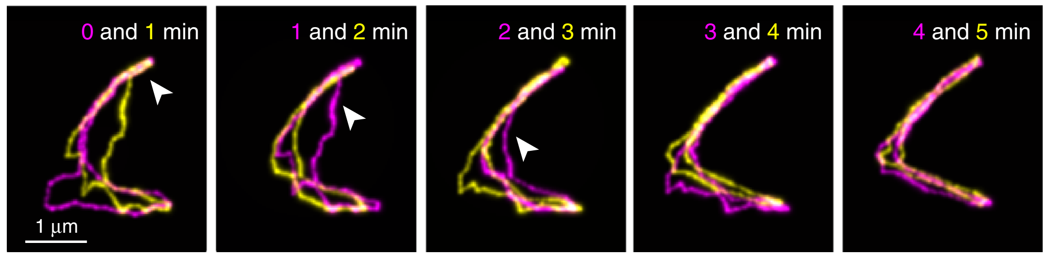
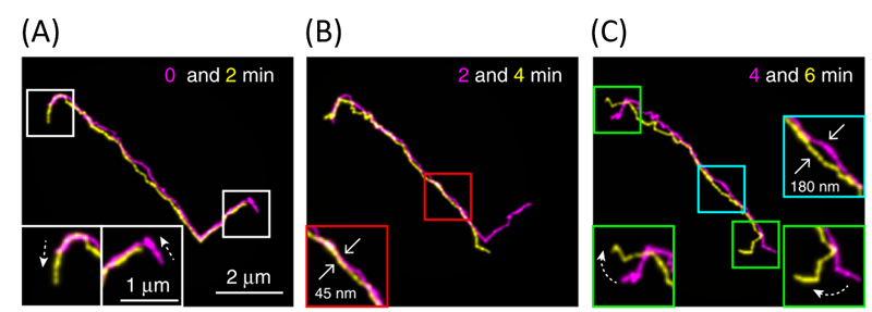
Figure 2. Fluorescent images of a linear DNA chain collected at different time points (indicated in the figure), overlapped for comparison. Insets show the enlarged views of the highlighted areas. (Adapted from the original paper.)
First, linear DNAs were used to confirm what has been known from reptation theory in great detail. Shown above in Figure 2 are images of a linear DNA as a function of time. Their results were consistent with theory. First, polymer chains traveled along virtual tubes that followed the contour of the chain (shown in white boxes in Figure 2A). Second, most of the polymer chain’s displacements were within the confinements of the virtual tubes, which had a diameter around 51–95 nm (shown in red boxes in Figure 2B). Further, they occasionally saw displacements of the DNA that exceeded the size of tube diameter (shown in cyan boxes in Figure 2C), known as constraint release in reptation theory. Finally, Abadi and coworkers observed that the chain-ends were able to move farther than the centers of the chains, which in turn creates a new tube for further DNA reptation (shown in green boxes in figure 2C). In reptation theory, this is called contour-length fluctuation.
However, there was one particular deviation from the theory found in the authors’ results. While the chain-ends were expected to move more freely than other parts of the chains, the chain-end motions were a lot faster than what is predicted by reptation theory. Therefore, the authors concluded that the motions at the chain-ends were beyond the scope of the reptation theory. These unexpectedly fast movements were not observed in previous experiments, in which only the chain as a whole was considered.
Figure 3. Both rows are fluorescent images of cyclic DNAs collected at different time points (indicated in the figure), overlapped for comparison. 3A shows amoeba-like motion, and 3B shows contracting of an open structure. More details can be found in the main text below. (Adapted from the original paper.)
The authors also observed cyclic DNAs using the same methods. As they are not linear, reptation theory fails to accurately explain their movements. The authors observed diverse motion of the cyclic DNAs. You may notice in Figure 3A that the cyclic DNA has a loop-like region, shown in the white boxes. They found that cyclic DNAs repeatedly contract and extend this region, resembling the motions of amoeba. In addition, as shown in the first panel of Figure 3B, some cyclic DNA molecules may start with an open structure. However, as time progresses, these open DNAs may contract into more linear forms and expand back into the open shape again. Thus, Abadi and coworkers were able to show two phenomena that cannot be explained by reptation theory, thus requiring it to be further refined.
The results of this paper support many of the conclusions of reptation theory; however, it does suggest that there is still a need to expand this otherwise well-accepted theory. By considering different geometries and shorter timescales, this theory will be more powerful as a predictor or explainer of novel polymeric material dynamics. Furthering the understanding of polymer dynamics will then help us understand polymer properties for use in a variety of applications that we see in our lives every single day.
[2] Polymers are molecules that are consist of repeating chemical structures.
[3] Super-resolution microscopy is a technique that lets us observe things that are smaller than the diffraction limit of ~200 nm, which is the limit that is imposed by the physics of light.
If you ever played tug-of-war in elementary school, you might remember that it isn’t the friendliest game. People fall over, hands get burned from holding on to the rope, and knees get scraped from falling on the ground. Although victory can be sweet, the injuries that come with it may make you never want to play the game again. Perhaps surprisingly, there is a similar ‘’tug-of-war” happening inside your body, as individual cells move around from one place to another in a process called cell migration. What’s more, this microscopic tug-of-war may help to heal those scrapes and bruises that happened in elementary school, and those that happen in your everyday life.
A single cell moves by detaching and reattaching from the substrate, or the surface it is on, as the cell expands and contracts. This movement exerts forces on the substrate. (These forces can actually be measured directly – this is the topic of a previous softbites post.) When many cells move together in a “cell sheet”, their motion becomes more complicated. Not only do cells push and pull on the substrate, but they also push and pull on the cells that surround them. In today’s study, Xavier Trepat and colleagues show that there is a “tug-of-war” between cells that causes them to migrate.
Previously, it was thought that only the cells at the very front of the mass of migrating cell, or the leading edge of the cell sheet, exert forces on the substrate. According to this picture, most of the cells get passively pulled along by the leading edge, and neither push nor pull on the substrate. By measuring the forces the cells exert on the substrate, Trepat and his colleagues discovered that, in fact, all of the cells are involved in pushing the cell sheet forward.
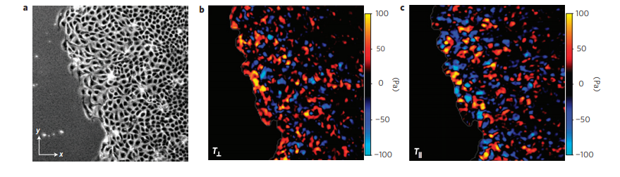
The researchers measured the forces in a moving sheet of cells, taken from canine kidneys, growing on a gel substrate using a technique called traction force microscopy. The first step of this technique is to track the displacements of different points within the substrate as the cells move. Then, the mechanical properties of the gel are used to calculate the forces on the substrate generated by this motion. The researchers mapped the value of these forces using different colors, with red and blue representing very strong forces and black representing zero force. They first looked at what happened at the leading edge of the cell sheet, as in Figure 1.
Figure 1. a. Image of the cell sheet, in which individual cells are outlined in white. The field of view is 700 microns by 700 microns. b. The forces that the cells exert perpendicular to the leading edge of the cell sheet. c. The forces that the cells exert parallel to the edge of the cell sheet. Bright red and blue colors indicate strong forces (up to 100 Pa of stress), while black color indicates low forces. (Images adapted from the original article.) The cell sheet’s expansion was recorded in a video as well.
The researchers separated the normal forces (Figure 1b) — those exerted by the cells perpendicular to the leading edge of the cell sheet, or in the direction of the cells’ motion — from the forces exerted parallel to the leading edge of the cell sheet (Figure 1c). The bright red and blue colors in Figure 1 show that cells well inside the cell sheet exert forces on the substrate. From this, they hypothesized that instead of having “follower” and “leader” cells, all the cells contribute into pushing and pulling the cell sheet as they move.
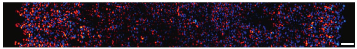
The researchers then looked at larger areas of the cell sheet, such as that shown in Figure 2. The bright colors near the edges correspond to strong forces, while the black spots show that the forces in the center of the cell sheet are weaker. This suggests that the cell sheet “tugs” both to the right and the left as it expands. As the cells exert forces on the substrate, they exert forces on each other. The cells pulling to the right and the left are similar to two teams pulling a rope in a game of tug of war. The sheet of cells is like a rope that grows in the direction of the tugging of the cells.
Figure 2. Forces exerted by a larger piece of the cell sheet. Bright red indicates strong positive forces and blue indicates strong negative forces, while black indicates low forces. The scale bar on the bottom right is 200 micrometers. (Image adapted from the original article.)
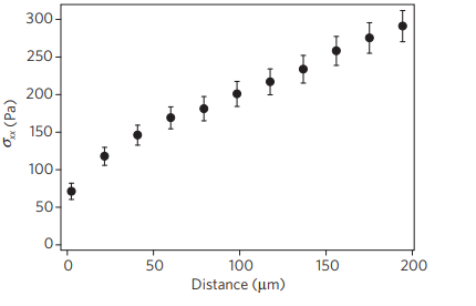
Next, the researchers wanted to understand how being tugged on by its neighbors affects the motion of individual cells: does the tug of war consistently pull a cell in a particular direction? Or is the cell equally likely to be pulled in any direction? To answer this question, Trepat and colleagues measured the average force exerted on a cell by its neighbors, as a function of the distance of that cell from the edge of the sheet. If each cell was moving independently, the average normal force inside the sheet would be zero – on average, no cell would be pushing or pulling any other cell to a specific direction. Instead, as shown in Figure 3, the average force was not zero, and was actually higher for distances farther from the sheet’s leading edge. In other words, the cell sheet is expanding from the inside more than it’s being pulled from the edge.
Figure 3. The average normal force exerted on a cell by its neighbors, $latex \sigma_{xx}$, is higher farther from the leading edge of the cell sheet. (Figure adapted from the original article.)
Each individual cell crawling on a substrate has little effect on its surroundings, but many cells acting together can exert forces on each other to guide the collective in a particular direction. As cells replicate, such as in a healing wound, this guiding helps the cells expand in directions where there is space to be filled. This study by Trepat and colleagues reveals for the first time the tug-of-war that allows the tissues in our bodies to grow and heal.
In my previous post on soft nanoparticles, you were introduced to polymer-based nanoparticles that could be used in biomedical applications, one of which is cancer therapy. These nanoparticles have a range of useful properties for cancer treatments, including their spherical shape and small size (~100 nm), both of which are similar to exosomes, small globules that are used in nature for transferring proteins between cells. Since cells naturally absorb exosomes, artificial particles with this size and shape should also be easy for cells to absorb, which means these particles could be used to deliver drugs into cells. While this idea sounds promising, it hasn’t worked out in practice — when drug-loaded polymer-based nanoparticles were injected into a tumor, subsequent tests showed that less than 1% of the injected dose entered the cancer cells. Since these particles were the correct size and shape, why didn’t they get inside the target cells?
One possibility is that the elasticity (or stiffness) of nanoparticles is to blame: scientists have suspected that this mechanical property can affect the ability of nanoparticles to squeeze themselves through the cell’s membrane. Unfortunately, it is difficult to test this hypothesis directly, because modifying the elastic properties of a nanoparticle generally requires modifying its chemical properties as well. To solve this problem, Peng Guo and coworkers designed a special kind of nano-objects — spherical nanolipogels — with tunable elasticity. In this paper, they proved for the first time that breast cancer cells take up soft, squishy particles more easily than they take up hard ones.
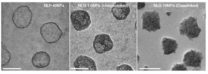
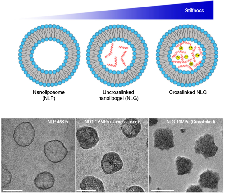
So what are nanolipogels? This type of nanoparticles is basically an altered version of a nanoliposome, a particle-like object that consists of a liquid water core surrounded by a layer of phospholipid molecules [1]. Guo and his colleagues created nanolipogels by filling the nanoliposomes’ liquid core with a polymer of tunable chemical structure. Nanolipogels have precise size (160 nm) and shape (spherical), and their elasticity can be made to vary without changing their other properties (see Figure 1).
Figure 1. Structures (top) and micrographs (bottom) of nanoliposomes and nanolipogels of increasing stiffness (higher values of Young’s modulus). (Image adapted from Guo’s paper.)
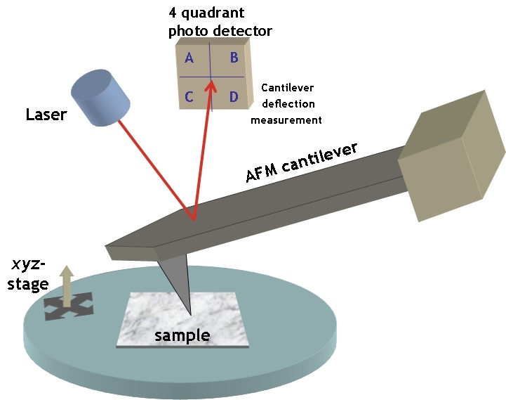
Figure 2. Experimental setup of an Atomic Force Microscope. The height of a sample’s surface is scanned by a tip on a moving cantilever and the cantilever deflections are detected by a laser light to give the samples topographic profile. (Image from simple.wikipedia.org)
To measure the elasticity of the particles they had produced, Guo and coworkers used a technique called Atomic Force Microscopy (AFM). AFM is commonly used to visualize soft materials by imaging the height of their surface through the deflection of a cantilever (Figure 2). In this paper, the researchers used AFM for a different purpose: to calculate the Young’s modulus — a measure of stiffness — of the nanoparticles. They did this by compressing the particles between the cantilever tip and a solid surface, allowing the researchers to measure the force required to deform the particles by some known amount. The relationship between the applied force, the degree of deformation, and the Young’s modulus is given by the Hertz equation [2]. What you need to remember is that the greater the modulus, the stiffer the particle.
The researchers created four different nanolipogels of different elasticity with Young’s moduli ranging from 1.6 MPa (roughly the stiffness of cork) to 19 MPa (the stiffness of leather), and a nanoliposome without polymer in the core with a Young’s modulus at 0.045 MPa (roughly the stiffness of gummy bears). After verifying that all 5 particles could successfully encapsulate drug molecules, they tested how well tumor cells could uptake each particle. To do so, they used breast cancer cells in the lab (in vitro cellular uptake) and attached fluorescent dye to the particles to determine whether they were inside or outside of the cells. They found that the stiffest nanolipogels were 80% less effective compared to the softest nanoliposome samples; in other words, five times more of the softer particles got inside the cells. In vivo tumor uptake studies, using live mice, similarly showed that the nanoliposomes had up to 2.6 times higher cellular uptake than the stiffest nanolipogels.
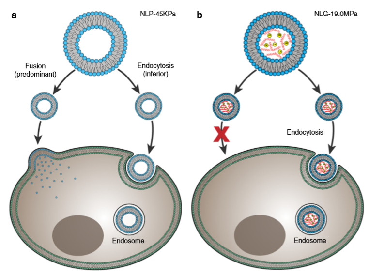
Why do the soft nanoliposomes enter the cells more easily? To understand the conclusion of Guo and colleagues, we need to think about how nano-objects enter a cell. Figure 3 shows two possible ways of doing this: 1. fusion, where nano-objects break up and join the cell membrane, or 2. endocytosis, where the whole object enters the cell by bending the cell’s membrane and getting covered in a membrane outer layer. Fusion needs less energy compared to endocytosis, where cell membrane bending and surface tension increase the energy. The researchers hypothesized that nanoliposomes use both fusion and endocytosis, with a preference for fusion (Figure 3a), while nanolipogels can only enter the cell through endocytosis (Figure 3b). This hypothesis was verified by using chemical compounds that prevented endocytosis from taking place; in all experiments, the cellular uptake of nanoliposomes was as high as before, while much fewer nanolipogels were detected in the cells, since they couldn’t enter through endocytosis.
Figure 3. The possible pathways of (a) nanoliposomes and (b) nanolipogels entering a cell. (Image adapted by the Guo paper.)
This study showed that a nanoparticle’s mechanical property, in particular, its elasticity, affects how it enters cells, a finding that could potentially have a tremendous impact on cancer treatment and diagnosis. The use of nanoliposomes, which are a synthetic equivalent of nature’s drug delivery systems, may also be used in the future to further understand how cellular processes, such as fusion and endocytosis, take place.
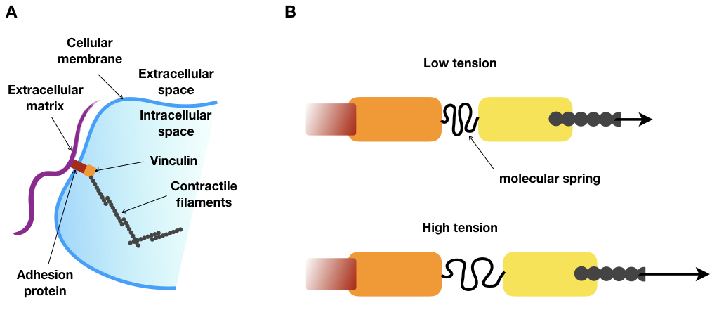
“USE YOUR LEGS!” That’s what might have been yelled at you the first time you went climbing. We are so used to walking or running that we don’t even think about how we do it. But when we face a new environment, such as a steep slope, we realize that finding the best strategy to move through space is not so easy. Now, imagine you are as small as few dozens of microns, without legs or arms, and you live in a viscous fluid. How would you move? This is the question biologists who are interested in cell movements have been trying to solve. By observing cells under a microscope, they saw that depending on their type or their environment, cells exhibit a wide variety of motion strategies. However, one thing never changes: cells need to exert forces on their environment to move. To do so, some kinds of cells create structures called focal adhesions. These structures are made up of several proteins, assembled on the outside of the cell. Like tiny bits of double-sided tape, their purpose is to stick the cell to whatever is nearby (see Figure 1). In slightly more technical language, focal adhesions connect the molecular skeleton of the cell to a substrate.
Figure 1. Movie of a moving cell with fluorescently labelled focal adhesions (from Berginski et al. 2011)
Cells can exert forces on their environment through focal adhesions. While it is possible to measure these forces outside the cell by engineering some force-sensing substrate [1], it is much trickier to understand what happens inside the cell. Accessing these forces inside the cells is the challenge Grasshoff and colleagues tackled in their 2010 paper.
In order to measure a force, the most straightforward method is to use a spring. A spring is a stretchable object for which, after calibration, we can relate its extension to the applied force. Therefore, a force can be measured by measuring the length of the spring. To measure the forces focal adhesions apply on the cell, one would need to inject tiny springs in the cells and connect them to the exerting-force structures.
To do this, the authors had the idea of taking advantage of a silk protein, produced by a spider, which is literally a molecular spring. Thanks to genetic tools, a part of the gene of this silk protein could be inserted within a gene called vinculin. The vinculin gene produces a protein that is an essential part of the focal adhesion structure. As shown in Figure 2A, vinculin connects the protein filaments of the cell skeleton to the outside of the cell (the extracellular matrix). The researchers engineered an artificial variant of vinculin that includes a molecular spring, derived from the silk protein, right in the middle of the naturally occurring vinculin molecule (see Figure 2B).
Figure 2.A. Schematic of focal adhesion. B. Schematic of the modified vinculin under low and high tension. Under high tension, the molecular spring is stretched. Red: adhesion protein, orange: vinculin head domain, yellow: vinculin tail domain, grey: contractile filaments. Arrows represent the magnitude of the tension.
After verifying that cells that are genetically modified to include the engineered focal adhesion protein behave normally, the next step was to measure the molecular spring extension. However, measuring distances at the molecular scale is not a piece of cake. For instance, the typical extension of such a spring is 6 nanometers, which is, by far, below the resolution of the best optical microscopes [2]. To circumvent this limitation, Grasshoff and colleagues took advantage of the Förster resonance energy transfer (FRET) effect to measure the distance between the two vinculin domains. The FRET effect takes place between two fluorescent molecules very close in space. A fluorescent molecule, when excited by a light at a precise wavelength, emits a light at a longer wavelength. But if a second fluorescent molecule is close enough, the first molecule (the donor) can directly transfer its energy to the second molecule (the acceptor). Then, the acceptor will emit light at an even larger wavelength than the donor’s. Consequently, the FRET intensity can be computed by measuring the relative emissions of the donor and acceptor molecules: the closer the acceptor is to the donor, the more energy the acceptor will absorb and re-emit. Furthermore, and importantly for this application, the efficiency of this process is very sensitive to the distance between the donor and the acceptor As a result, the distance between the two molecules can be measured with great precision (sub-nanometer) by measuring the intensity of the FRET effect. Therefore, the authors further engineered the vinculin protein by placing the molecular spring between two fluorescent molecules (Figure 3, yellow and red circles) that were capable of undergoing the FRET effect to measure the extension of the molecular spring.
Figure 3. Förster resonance energy transfer (FRET) effect in the modified vinculin of a focal adhesion under low and high tension. The excitation light of the donor molecule (yellow circle) is shown in green and the emission light of the acceptor molecule (red circle) is shown in red.
At this point, the authors had a method for measuring the tension intensity across vinculin molecules just by looking at the FRET intensity. In this way, they could generate a tension map across the contacts of the cell with its environment. They saw that focal adhesion under high tension leads to a growth of the size of the focal adhesion which relieves it from its high tension. Perhaps surprisingly, they also showed that regions where the contact is extending (protruding areas) are under higher tension than regions where the contact is receding (retracting areas), as shown in Figure 4.
In this paper, the authors developed a new technique to measure forces inside cells. By conducting single-molecule experiments, they even could calibrate their engineered molecular spring and relate the FRET intensity to absolute values of forces (in the order of a few piconewtons [3]), paving the way to a whole class of new FRET-based force sensors with different stiffnesses, which can now be used in other structures inside cells.
Everything started with adding a spider silk gene in a cell. Such mutant cells have the amazing power of shading light on the cellular force machinery. But “with great power, comes great responsibility” as another spider mutant has once been told.
Figure 4. The FRET index (ratio of donor to acceptor fluorescence) reveals the state of tension through vinculin across a cell. Close-ups retracting areas (R1 and R2) show a high FRET index, ie. a low tension, and protruding areas (P1 and P2) show a low FRET index, ie. a high tension (adapted from Grashoff et al.).
[1] These techniques are called traction force microscopy. The deformation of calibrated substrate (either a gel or micropillars) is measured to calculate the forces exerted by the cell. [2] Classical optical microscopes have a typical resolution of around 200 nm. New techniques of super-resolution microscopy reach a resolution of a few dozens of nanometers. [3] To give you a sense of this order of magnitude, when you hold a pen of, let’s say 10 g, you apply a force of 0.1 N. At the cellular level, cells exert on their environment forces in the order of dozens of nanonewtons (according to this study). At the molecular level, DNA has been manipulated applying forces in the same range as the vinculin tension: 1-100 pN (according to this study).
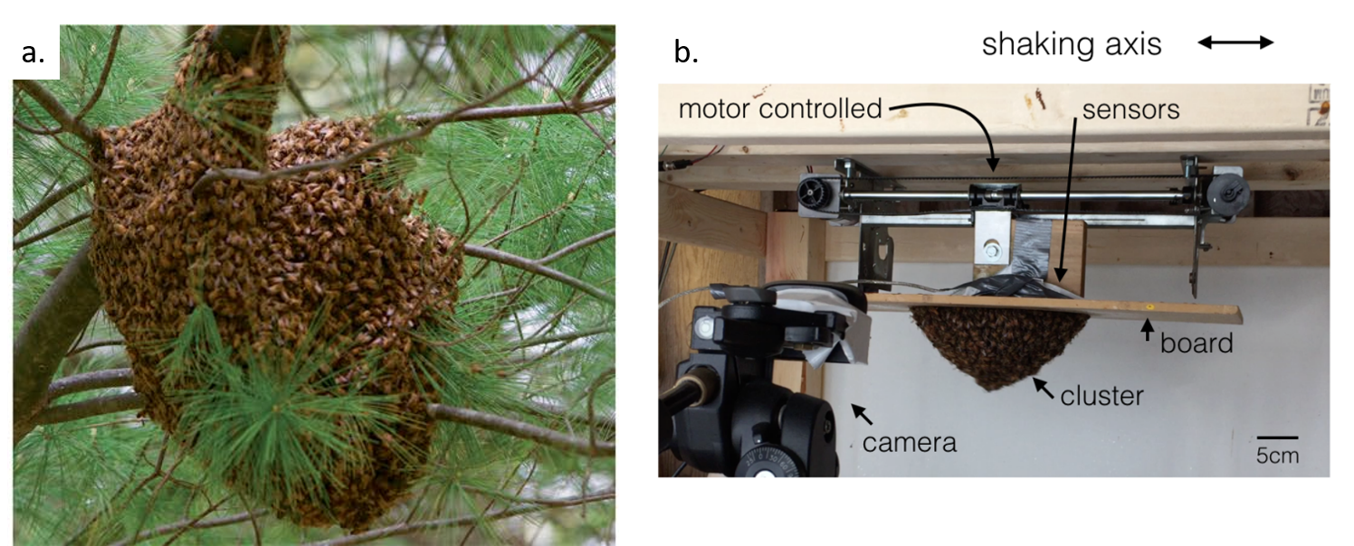
A honeybee colony can only exist when many individual bees cooperate. When a hive becomes too crowded, about 10,000 of the workers and a queen leave the hive to form their own colony. While the scout bees are searching for a new nest site, the rest of the bees are exposed to all of the dangers of the outside world, such as predators and storms, and have to stick together for protection. They form a “cluster”, which hangs on a nearby tree branch (as in Figure 1a) until a new suitable nest site is found. Sometimes, beekeepers hang these clusters from their faces as a “bee beard”.
In this study, Orit Peleg and colleagues investigated how these bee clusters stick together against the forces of gravity and the wind by shaking them and tracking how the shape of the cluster changed. Their experimental setup consisted of a board attached to a motor that shook it horizontally at frequencies between 0.5 and 5 Hz and accelerations up to 0.1 times gravitational acceleration. Peleg and colleagues put a queen bee in a cage attached to the board, leading the rest of colony to cluster around her, as shown in Figure 1b. Once the cluster formed, the researchers turned on the shaking and filmed how the bees behaved.
Figure 1. a) A bee cluster in the wild. The worker bees are protecting the queen until they find a new hive. b) A bee cluster in the lab, with the queen attached to the top board in a cage. Figure adapted from original article.
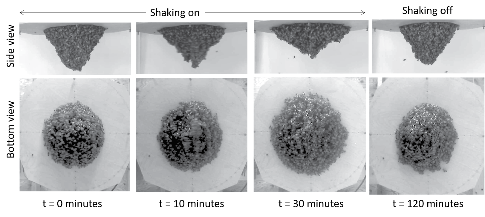
As the bee cluster was shaken horizontally, its tip swung from side to side at about 1 Hz, or one cycle per second. Peleg and colleagues tracked the bees moving from the tip of the cluster to the base as the cluster flattened over about 30 minutes. A flatter cluster does not swing nearly as much as an elongated one. Once the shaking was turned off, the cluster elongated again after 30 minutes to two hours, longer than it took the cluster to flatten. This is shown in Figure 2.
Figure 2. A honeybee cluster adapting to shaking filmed from the side and the bottom over time. While the shaking is on, the cluster spreads out along the base, and becomes shorter. When shaking is turned off, it returns to its original form. Figure adapted from original article.
Peleg and colleagues observed that individual bees responded to the variations in strain near them. At the base of the cluster, the strain was high, since the base bore the load of the entire swinging cluster. The bees at the base stretched their limbs to hold the rest of the cluster as it swung back and forth. The strain at the tip of the cluster was lower, since the bees there did not have to stretch as much to hold on. As more bees reached the base of the cluster, it flattened, making it swing less and decreasing the local strain on all the bees. The cluster was much flatter after 30 minutes of shaking, as in Figure 2. The bees at the base then didn’t have to stretch as much to hold on, and the cluster was safe from being torn apart. Even though an individual bee moved towards a greater strain, which may have been less comfortable for it, this collective bee behavior ultimately decreased the strain on the entire colony.
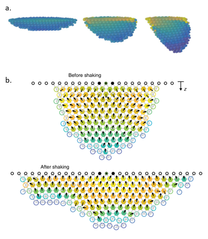
The researchers hypothesized that when a bee experienced a “critical strain”, a high value that might endanger the cluster, it moved to where the strain was higher — up towards the base —changing the cluster’s shape. To show that moving in the direction of increasing strain is a possible explanation for how the cluster flattens, Peleg and colleagues simulated honeybee clusters of different shapes under horizontal shaking (Figure 3). Each bee was modeled as a spherical particle experiencing gravity and attraction to neighboring bees. The simulated bees could not overlap with each other.
For their first simulation, the researchers simulated an entire cluster in 3D with stationary bees subject to horizontal shaking. They wanted to investigate the relationship between cluster shape and the strain. In this simulation, longer bee clusters experienced a higher strain when they were shaken, as shown by the color gradient in Figure 3a, with yellow corresponding to a higher strain than blue.
A second set of simulations allowed bees to break their connections with their neighbors and move in the direction of increasing strain if their neighboring strain was above a critical value. As expected, bees moved towards the base when shaking was simulated, and the cluster flattened out forming a shape similar to what was observed with real bees in Figure 2, shown in Figure 3b.
Figure 3. a) Three clusters simulated with horizontal shaking, from flat to elongated. Longer clusters have much stronger strains at the base. Blue colors correspond to lower strains while yellow corresponds to high strain. b) When shaking is turned on, simulated bees move towards higher strain (in the direction of the arrows) and flatten the cluster. Red and yellow colors correspond to higher strains. Figure adapted from original article.
This behavior lets bees keep the queen safe and the colony together on the tree when the cluster swings side-to-side in the wind. The cooperation of bees following simple rules lets the colony survive until it finds a new home.
For the most part of biology, it is form that follows function. Proteins are a perfect example of this — they are made of a sequence of amino acids (the protein building units), which are synthesized by the ribosome. Once synthesized, the long strings of amino acids fold up into a particular 3D shape or conformational state. Proteins take less than a thousandth of a second to attain their preferred conformational state (called “native state”) that — if nothing goes wrong — ends up being the same for a given sequence. This process is called protein folding. Explaining how a protein finds its folding preference out of all possible ways in such a short time is a longstanding problem in biology.
But, how do scientists know if – and when – a protein is in its folded state? The most straightforward way to do this is by observing its function — the way that a protein performs some biochemical task within the cell. If the protein is functionally active, then it has achieved its proper structure. However, most proteins are too small to observe directly without damaging the cell. To solve this problem researchers frequently use Green Fluorescent Protein (GFP), a protein that glows when it is hit by light of a specific wavelength. By attaching GFP to other proteins, researchers can see exactly where those proteins are at different timepoints. GFP’s stability, lack of interaction with other proteins, and non-toxicity make it an extremely popular candidate for visualizing protein localization. In other words, one “function” of GFP is to fluoresce. Today’s paper seeks to understand how structure correlates with function in GFP, one of biology’s most important tools.
To control the folding process, the authors used dual optical tweezers to mechanically stretch and relax the protein. Optical tweezers — as the name suggests — manipulate the position of particles (beads) using laser light. These beads are typically in the size range of micrometers. To apply forces on the GFP, the beads are attached to the protein via DNA “handles,” so that a DNA strand attached to the protein will stick to the DNA strand attached to the bead. These strands are then bound together ensuring that the force on the beads is transferred to the GFP. The construct looks as follows:
Bead – DNA – Protein – DNA – Bead
When the beads move apart, the protein is stretched to its maximal possible length (also called its contour length) and is unfolded, but when the beads get closer together, the protein folds back to its preferred structure. This process is illustrated in Figure 1.
Figure 1: The beads (circles) at each end are manipulated by laser beams and move back and forth. The DNA handles (purple) are attached to the GFP protein (green) that folds and unfolds turning to a functionally active and inactive state, respectively.
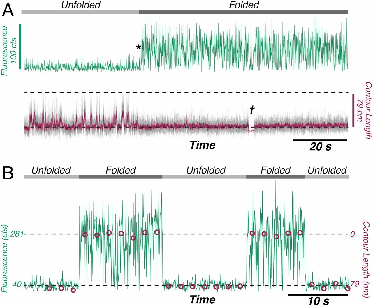
The authors observed that during unfolding, the GFP protein has undergone two intermediate states before unfolding completely. After unfolding, the beads were brought closer together and the protein folded itself back through the intermediate stages. The GFP molecule stopped emitting light when it was unfolded, which was expected. However, it started fluorescing only when it was completely in its folded state. This important finding showed that this protein is functionally inactive in any of the intermediate folding stages. The authors also observed that this process is reversible; they could unfold and refold the GFP molecule multiple times (see Figure 2).
Figure 2: Fluorescence signals of the GFP protein as it cycles through the unfolding and folding states. (A) The unfolded protein (light gray line) emits very little light (green signal) and its length fluctuates (purple line). Once the protein refolds (*) it emits more light and its length becomes shorter and consistent (dark gray line). † is the point where the force and state conformation are correlated(B) Cycled transition from dark (unfolded) to bright (folded). The purple circles represent the average contour length of each time. (Image adapted from Ganim’s and Rief’s paper).
These findings contribute towards understanding the functionality of proteins that could be used as in vivo optical sensors in force transduction. This work also opens up new avenues in studying biomolecules at the single-molecule level, such as DNA-protein complexes that can induce changes in conformation. Although the experiment only pulled the protein along one axis, this technique could be extended to pulling in several directions at once. If one could control the applied force in 3D, then it could be possible to gain more information on how exactly the protein folds and/or what happens during that process.
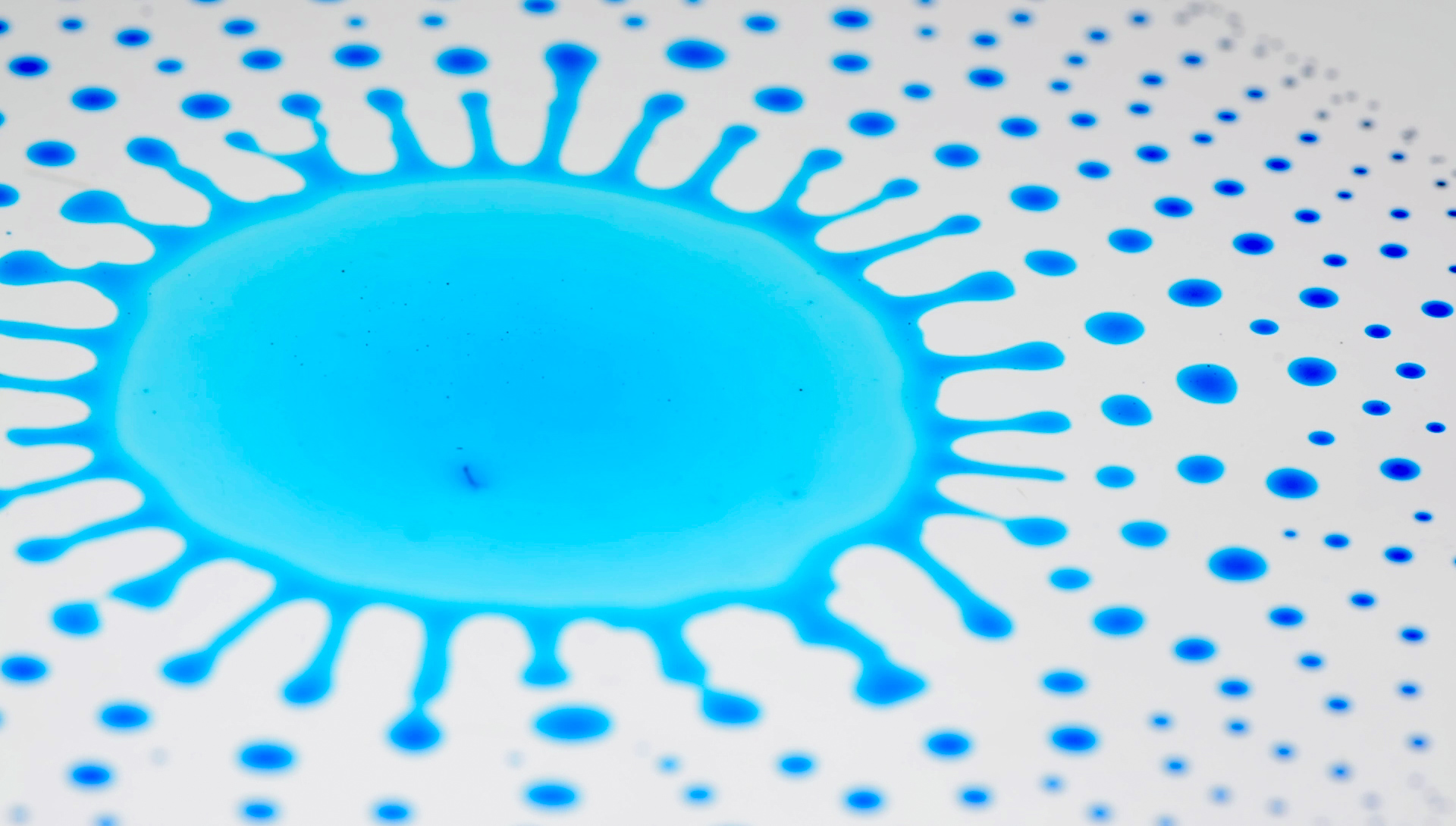
We are surrounded by phenomena caused by the scattering of light. When enjoying a sunny day at the seaside, like in the photo at the top, why is the sky blue? Blue light scatters more than red light. Why is milk opaque? Protein and fat particles scatter light. If you are reading this with blue eyes, your eye color is due to light scattering. Scientists use the same general scattering principle to study the structure of soft materials using the scattering of well-defined radiation. Scattering measurements reveal structures between an ångström and hundreds of nanometers, an important region for studying soft matter. Just as the color of the sky results from light scattered by air molecules, the scattering of X-rays and neutrons tells us about the size and shape of compounds in soft materials along with their interactions, and I will focus on these two types of radiation.
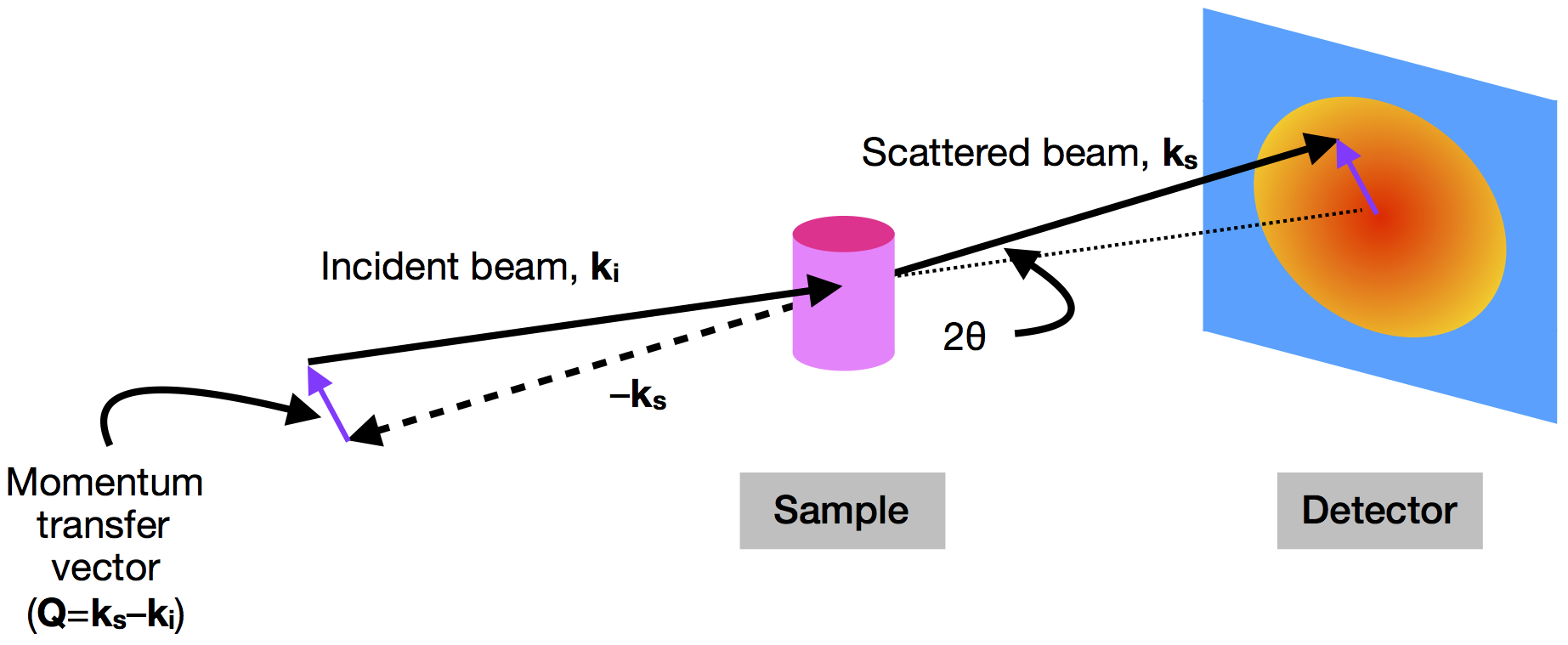
In a small-angle scattering experiment (SAXS when using X-rays and SANS when using neutrons), a sample (whether solution, dispersion, or solid) is placed between an incoming beam of radiation and a detector (see Figure 1) [1]. The detector measures the scattering intensity as a function of angle, which in turn can be related to the size and shape of the sample’s components.
Scattering intensity is quantified as a function of the momentum transfer vector (or scattering vector) $latex \mathbf{Q}$, which is simply the difference between the momentum of the incoming beam ($latex \mathbf{k_i}$) and the scattered beam ($latex \mathbf{k_s}$). The magnitude of $latex \mathbf{Q}$ (equal to $latex (4 \pi \sin{\theta}) / \lambda$) depends on the scattering angle ($latex 2 \theta$) and the wavelength of the radiation ($latex \lambda$) [2].
Figure 1. The geometry of a small-angle scattering instrument. An incident beam of X-rays or neutrons (with momentum $latex \mathbf{k_i}$) is scattered by a sample with an angle of $latex 2 \theta$. The scattered beam (with momentum $latex \mathbf{k_s}$) is then detected at a point beyond the sample. The difference in momentum between the incident and scattered beams is $latex \mathbf{Q}$. (Image produced by the author.)
The relationship between the magnitude of $latex \mathbf{Q}$ and the length scale being investigated ($latex d$) is given by the equation $latex Q = 2 \pi / d$, and this inverse relationship to distance is why measurements as a function of $latex Q$ are said to be in reciprocal space. (This relationship comes from Bragg’s law for crystals [3].) In real space, the arrangement of objects is described by the distances between them. In reciprocal space, the same arrangement would be given by $latex Q$. The scattering process is essentially a Fourier transform [4], a mathematical procedure to convert waves to frequencies, making it possible to go between real and reciprocal spaces.
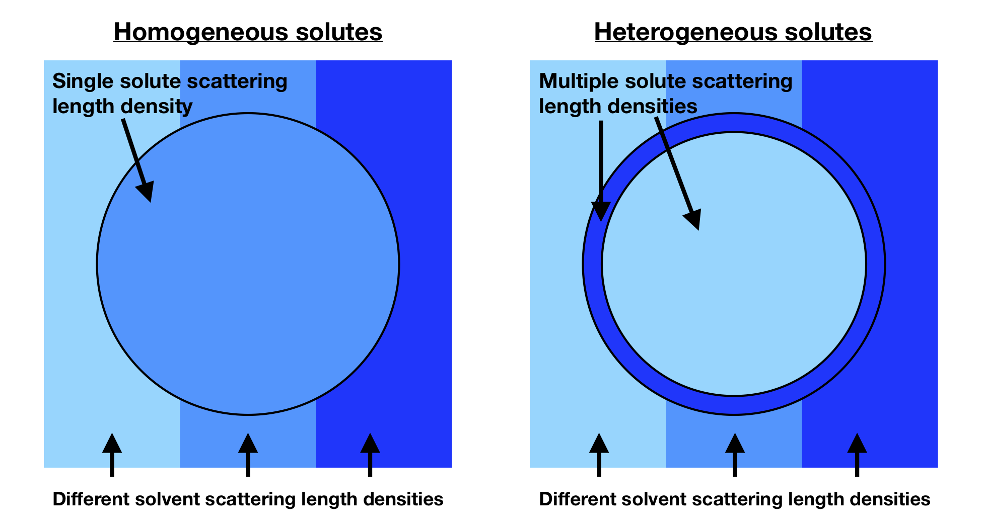
Now, having established some of the fundamentals of waves and scattering, we need to think about how radiation interacts with materials. This interaction determines the way that scattering data look and also what information you can obtain. Specifically, X-rays interact with electrons, and neutrons interact with nuclei. The magnitude of the interaction is quantified by the amount per volume (the “scattering length density”), and a difference in scattering length density between solutes and solvents results in detectable scattering. The scattering length density can be thought of as the “refractive index” for neutrons or X-rays. Figure 2 shows the general idea of contrast for any scattering experiment, with a comparison between homogeneous and heterogeneous solutes. When the color of the solvent and particle are the same shade of blue (meaning they have the same scattering length density), there is no scattering from that component. When the colors are different (meaning that they have different scattering length densities), there is now scattering.
Figure 2. Schematic of how the contrast between solutes (circle) and solvents (surrounding) for solvents and solutes with different scattering length densities gives rise to scattering. When the two colors are matched, which is possible for homogeneous solutes (left), there is no scattering. For heterogeneous solutes (right), there is no one solvent that can match the entire particle. (Image produced by the author.)
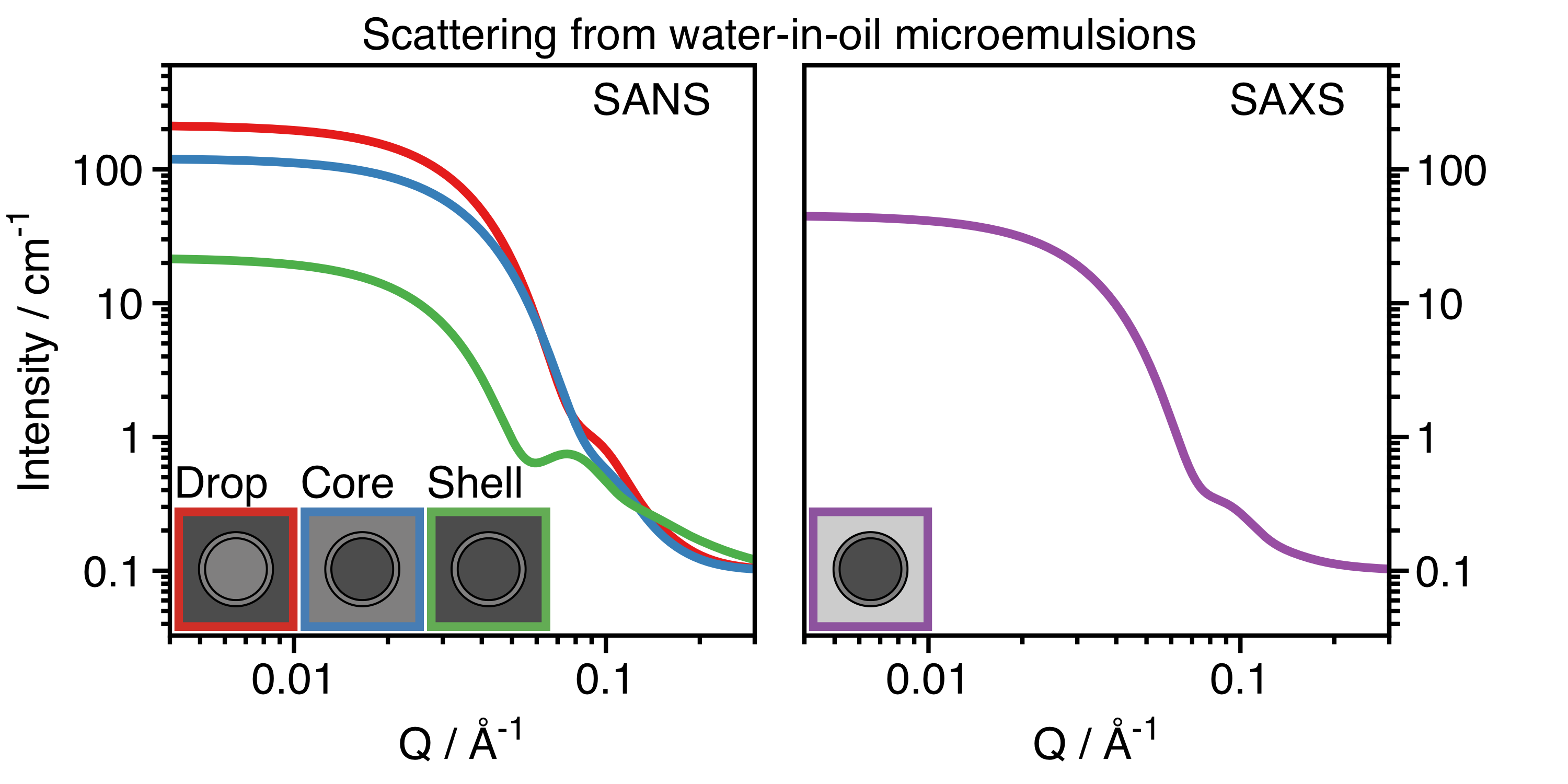
Interactions between X-rays and materials are fixed by their composition. However, neutrons interact differently with different isotopes of the same element. One particularly useful difference, especially for soft organic materials, is for structures with protons (1H) and those where protons are exchanged for deuterons (2H or D) [5]. It is possible to detect scattering from specific parts of complex systems by tuning the contrast of different components using solvents with different contrasts, as shown in Figure 2. Figure 3 shows calculated SANS (left) and SAXS (right) curves from chemically identical but isotopically distinct microemulsions, which are nanometer-sized droplets of water that are surrounded by surfactants in oil [6]. For the SANS curves, the dark grey areas represent deuterated oil or water (called D2O or heavy water), and the light grey areas represent standard hydrogenous oil or water. Multiple contrasts are required for a heterogenous particle, because no single solvent can match the whole particle (Figure 2, right). The curves are all different, but the actual structure of the microemulsion is always the same. It is only the contrast that differs. A precise determination of the structural dimensions of the microemulsion can be determined by analyzing all the data together, which gives more certainty than considering any one alone.
Figure 3. Scattering intensity as a function of the $latex Q$ for water-in-oil microemulsions calculated for SANS (left) and SAXS (right). For the three SANS curves measured, the dark grey regions are deuterated water (D2O) or deuterated oil, and the light grey regions are standard water (H2O) or oil. For drop contrast (red), you detect surfactant and water. For core contrast (blue), you detect water only. For shell contrast (green), you detect surfactant only. For the SAXS curve (purple), the contrast is fixed, and the water core dominates. (Image produced by the author.)
Scattering data is analyzed by comparing experimental data to known equations for how different shapes should scatter radiation as a function of $latex Q$. Luckily, many models are already known [7] for various shapes. However, as structures are determined somewhat indirectly from the scattering data, complementary information from other techniques, such as microscopy, is frequently obtained as well. The equation relating the shape and scattering as a function of $latex Q$ is called the “form factor”, an intraparticle property. For example, the curves in Figure 3 were all calculated using a form factor for a particle consisting of a spherical core surrounded by a shell of another material. At the extremes of $latex Q$, approximations can be used to calculate the size (at low-$latex Q$) and the interfacial roughness (at high-$latex Q$). In addition, the size distribution usually must be considered. In the example in Figure 3, the radii of the cores do not have a single value. There is a size distribution of about 20%.
For more concentrated dispersions or for more strongly interacting systems, the interactions between the particles must be considered. In these cases, an interparticle property called the “structure factor” contributes to the shape of the scattering curves. It can be calculated for particles that are considered to interact as hard spheres, charged spheres, or attractive spheres. Often samples are studied dilute to avoid the structure factor contribution. However, for systems that are necessarily concentrated or charged, it must be accounted for.
In this post, I focussed on the fundamentals of scattering with examples from nanoparticle dispersions in dilute conditions. However, these are not the only kind of soft materials that can be studied. Polymer solutions and blends, complex fluids, liquid crystals, gels, and a variety of biological materials (such as proteins and nucleic acids in solution or lipid bilayers) can be studied using small-angle scattering. The properties of soft materials often emerge out of their structures. By characterizing them in a quantitative way, scientists can determine the relationships between structures and their functions. Using small-angle scattering, we can not only better understand materials but also better predict ways of improving them. Small-angle scattering should be one of the tools employed by everyone interested in soft materials.
The featured image at the top is a photo of Bellevue Beach in Klampenborg in Copenhagen, Denmark. (Image taken by the author.)
[2] The angles being scattered are truly small, typically on order of 1° or less. By using $latex Q$, it is both the wavelength and angle that are important, and conveniently measurements performed using different wavelengths can be directly compared. ^
[3] Bragg’s law gives the conditions that a wave is diffracted by a series of planes. In a crystal diffraction measurement, peaks are observed in the data when Bragg’s law conditions are met. In a scattering measurement, where Bragg peaks are seldom observed, the relationship between $latex Q$ and $latex d$ is useful as a ruler for the length scale that is being examined. ^
[4] A Fourier transform is a mathematical operation that turns a periodic function, like a wave, into a probability of different frequencies. If, for example, you had a wave with a single wavelength, its Fourier transform would give a 100% probability at that wavelength. ^
[5] Deuterium is the heavy isotope of hydrogen with one neutron and one proton. ^
[6] A microemulsion is not just a small emulsion. Although, both are dispersions of two immiscible liquids, typically stabilized by a surfactant. A microemulsion is thermodynamically-stable and, in the case of a water-in-oil rather than oil-in-water, can be thought of as water-swollen surfactant micelle. Data for Aerosol OT-stabilized water-in-oil microemulsions can be found in the PhD thesis “Phase behaviour and interfacial properties of double-chain anionic surfactants” by Sandine Nave (University of Bristol). ^
Look inside a glass of milk. Still, smooth, and white. Now put a drop of that milk under a microscope. See? It’s not so smooth anymore. Fat globules and proteins dance around in random paths surrounded by water. Their dance—a type of movement called Brownian motion—is caused by collisions with water molecules that move around due to the thermal energy. This mixture of dancing particles in water is called a colloid.
Colloids are one of the classic topics in soft matter, a field of physics that covers a broad range of systems including polymers, emulsions, droplets, biomaterials, liquid crystals, gels, foams, and granular materials. And while I can keep adding items to this list, I can’t give you a precise definition for soft matter. I’ve never seen a completely satisfying definition, and I’m not going to even attempt to provide that here. But I can give you a taste of some of the definitions, and I hope you’ll come away with the feeling that you sort of know what soft matter is.
The phrase “soft matter” brings to mind pillows and marshmallows. These things fall under physicist Tom Lubensky’s definition (given in a 1997 paper) of soft materials as “materials that will not hurt your hand if you hit them.” And while many materials in soft matter are too squishy to hurt you, some of them might—cross-linked polymers can be pretty hard. And what about colloids? Slapping milk won’t hurt, but it also seems strange to call milk soft.
To understand what the “soft” refers to in “soft matter”, we first have to know where the name came from. The French term “matière molle” was coined in Orsay around 1970 by physicist Madeleine Veyssié, who worked in the research group of one of the founding fathers of soft matter, Pierre-Gilles de Gennes. The phrase apparently started as a private joke within the de Gennes group (don’t ask me what it meant), and the English translation of “soft matter” was popularized by de Gennes in a lecture he gave after winning the Nobel prize in 1991. De Gennes wrote that soft matter systems have “large response functions”, meaning that they undergo a large (don’t ask me how large) change in response to some outside force. So it seems we’re meant to take “soft” to mean something closer to “sensitive”, not necessarily soft in a tactile sense.
Now we can think about why colloids are soft from a different perspective. Remember that milk droplet under the microscope? The fats and proteins move around in the droplet due to thermal energy in the water; they are “sensitive” to the forces caused by thermal energy.
But even this “large response functions” idea doesn’t describe everything in soft matter. Some topics often considered a part of the field are concerned with general mathematical concepts instead of particular materials or systems. Take, for example, particle packing—the way particles arrange themselves to fit into confined spaces. Studying how particles can be arranged to pack on a curved surface is a mathematical problem and isn’t directly related to large response functions. However, since classic soft matter systems such as colloids are made up of particles you might want to pack, it makes sense to include packing as part of the field.
For every definition you give for soft matter, you can find a system that doesn’t quite fit. In an APS news article from 2015, Jesse Silverberg described soft matter as “…an amalgamation of methods and concepts” from “physics, chemistry, engineering, biology, materials, and mathematics departments. The problems that soft matter…examines are the interdisciplinary offspring that emerge from these otherwise distinct fields.” So maybe it’s not that important to have a rigid definition for soft matter; maybe its indefinability should be part of its definition. Soft matter is a field where the lines between traditional scientific disciplines are becoming ever more blurred—or, rather, soft.


![Berginski M, Vitriol E, Hahn K, Gomez S [CC BY 2.5 (https://creativecommons.org/licenses/by/2.5)], via Wikimedia Commons](https://softbites.org/wp-content/uploads/2019/02/high-resolution-quantification-of-focal-adhesion-spatiotemporal-dynamics-in-living-cells-pone.0022025.s014.ogv.jpg)