Much of how DNA and proteins function depends on their conformations. Diseases like Alzheimers’ and Parkinsons’ have been linked to misfolding of proteins, and unwinding DNA’s double-helix structure is crucial to the DNA self-copying process. Yet, it’s difficult to study an individual molecule’s mechanical properties. Manipulating objects at such a small scale requires tools like optical and magnetic tweezers that produce forces and torques on the order of pico-Newtons, which are hard to measure accurately. One way around these difficulties is by modeling a complicated molecule as an elastic fiber that deforms in predictable ways due to extension and rotation. However, there are still many things we don’t know about how even a simple elastic fiber behaves when it is stretched and twisted at the same time. Recently, Nicholas Charles and researchers from Harvard published a study that used simulations of elastic fibers to probe their response to stretching and rotation applied simultaneously. The results shed light on how DNA, proteins, and other fibrous materials respond to forces and get their intricate shapes.
Before continuing, I would recommend finding a rubber band. A deep understanding of this work can be gained by playing along with this article.
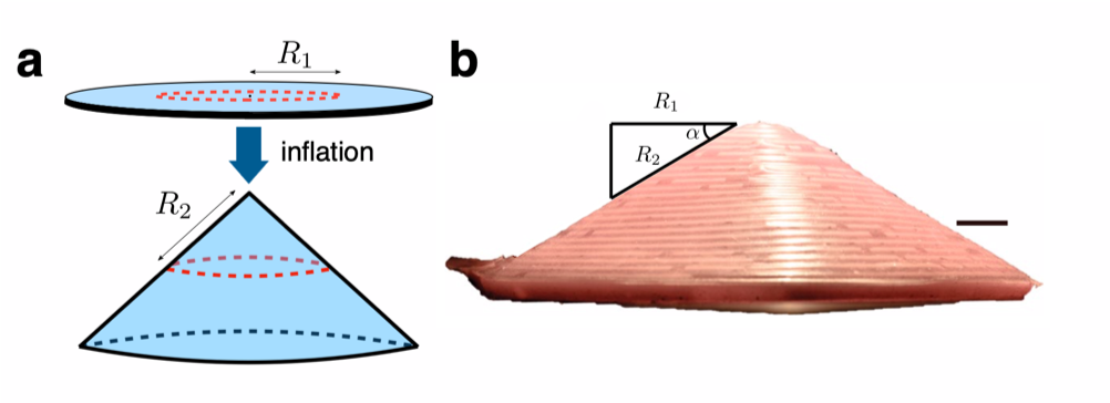
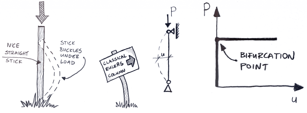
Long and thin elastic materials, (like DNA, protein, and rubber bands), are a lot like springs. You can stretch or compress them, storing energy in the material proportional to how much you change its length. However, compressing them too much may make the material bend sideways, or “buckle”. It might be more natural to think of this process with a stiff beam like in Figure 1, where a large compressive load can be applied before the beam buckles. But since your rubber band is soft and slender, it buckles almost immediately.
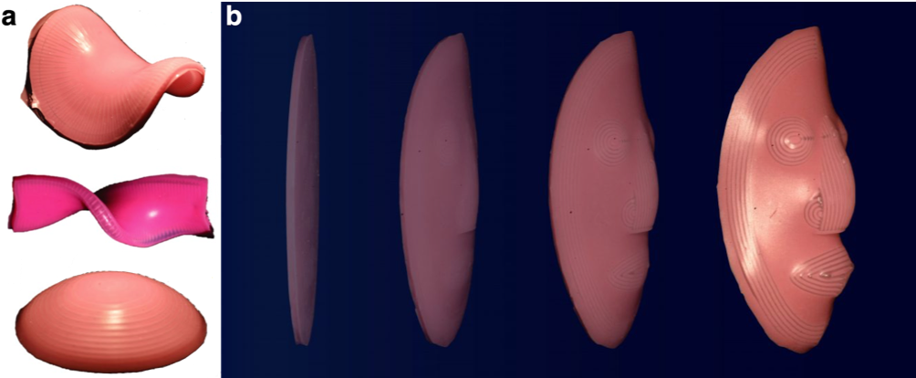
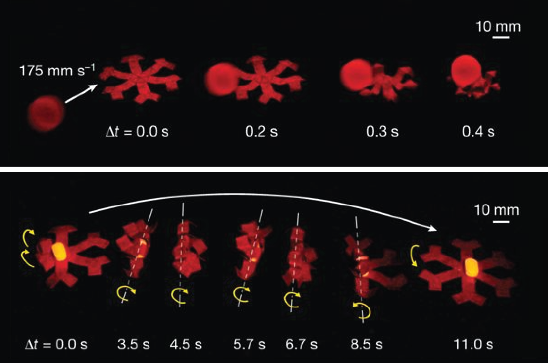
Likewise, twisting your rubber band in either direction will store energy in the band proportional to how much it’s twisted. And, like compression, twisting can also cause it to deform suddenly. Instead of buckling, the result is a double-helix-like braid that grows perpendicular to the fiber’s length, as shown in Figure 2. An important caveat is that the ends of the rubber band are allowed to come together. But what happens when the ends of the band are fixed?
Fixing the ends of a rubber band forces it to stretch as it twists. When this happens, a different kind of deformation can occur that combines extending, twisting, and bending the fiber. By stretching and bending simultaneously, the band forms a solenoid that is oriented along the long-axis of the band, reminiscent of the coil of a spring. An example of the solenoid shape appears in Figure 3.
All of the phenomena described above can be seen by playing with rubber bands, yet a quantitative understanding of how these states form and how to transition between them has remained elusive. To tackle this problem, Charles and coworkers used a computer simulation to calculate the energy stored at each point along an elastic fiber when it is stretched and twisted. The simulated fiber was allowed to deform and search for its lowest energy configuration, a process critical to navigating the system’s instabilities and finding the state you would expect to find in nature.
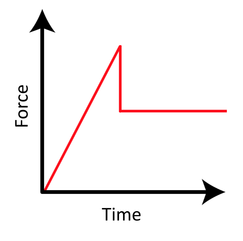
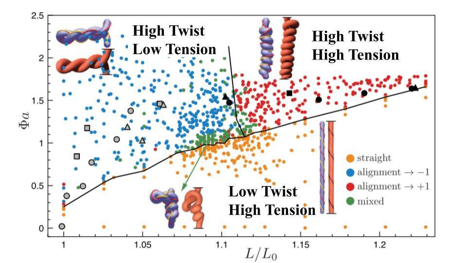
Figure 4 summarizes some of the different conformations attained by a fiber that is first stretched, then twisted to different degrees. We can see how a fiber with the same tension and different degrees of twist can lead to any one of a wide range of conformations. For instance, a fiber remains straight (yellow dots) when it’s stretched to a length $latex L$ that is 10% longer than its original length $latex L_{0}$ $latex (L/L_{0} = 1.1)$ until it is twisted by $latex \Phi a \approx 1$, where $latex \Phi a$ is the degree of twist multiplied by the fiber’s width divided by its length. Above this value of $latex \Phi a$, the simulated fiber twists into the braided helix structure seen in Figure 2 (blue dots). Likewise, when $latex L/L_{0} = 1.2$, the fiber remains straight until it has a much higher twist, $latex \Phi a \approx 1.5$, where it forms a solenoid (red dots).
Considering the vast understanding of the universe that physics has given us, it may be surprising that there is so much left to learn from the lowly rubber band. While it’s fun to play with, understanding the way fibers deform could help researchers understand all sorts of biological mysteries. For instance, your DNA is a unique code that contains all of the information needed to create any type of cell you have, but depending on where the cell is in your body, that same DNA only makes some specific cell types. The cell can do this by selectively replicating sections of its DNA while ignoring others. One way it does this is by hiding away certain regions of DNA through folding. Exploring the way simple elastic fibers deform could help explain the way DNA knows how to make the right cells, in the right places.