Original paper: Synthetic beta cells for fusion-mediated dynamic insulin secretion
Type 2 diabetes currently affects ~ 410 million people worldwide. It is a chronic condition caused by dysfunctioning beta cells in the pancreas. Beta cells normally secrete insulin in the pancreas to regulate blood glucose levels, and the loss of beta cell function can lead to hyperglycemia (i.e. high blood sugar), a condition with complications such as blindness and heart disease. The traditional invasive treatment involving direct insulin injection is a painstaking, never-ending process as it doesn’t properly regulate the dynamics of beta cells, just treats the symptoms. Modern treatments involve cell therapy in which functioning beta cells are transplanted from a healthy person, but this therapy faces serious challenges such as finding the right donor and suppressing the immune system after the transplantation. In this post, you will read how Chen and co-workers design an artificial version of beta cells that bypass the shortcomings of conventional cell therapy.
In our body, beta cells in the pancreas are responsible for monitoring and balancing our blood sugar level. When glucose levels are low (hypoglycemia, low sugar levels), these cells rapidly secret a polymeric (see note [1]) form of glucose. With high glucose levels (hyperglycemia) a hormone called insulin is secreted to bring down the concentration of sugar in the blood. Any disturbance to these cells, either through the body attacking itself (Type I diabetes, see note [2]) or genetic risk factors, can compromise the function of the beta cells, resulting in hypo- or hyperglycemia.
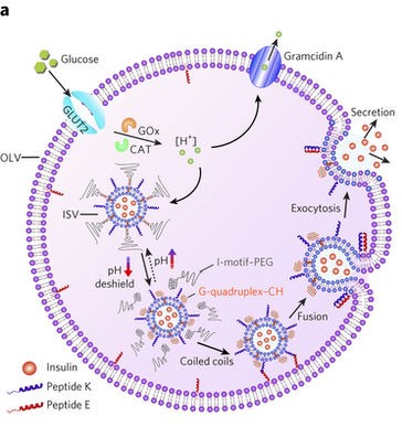
In this study, the researchers mimic the cell’s machinery in beta cells that sense sugar and signal a response inside the cell. This artificial system features two differently sized lipid vesicles (see Figure 1). The larger vesicle is about a micron in size (millionths of a meter) and is called the outer layer vesicles (or OLVs). It acts as the body of the artificial beta cell, encompassing the necessary machinery to regulate the insulin release. The second, smaller lipid vesicles, a thousand times smaller than the OLVs, are held inside the OLVs and are thus called inner layer small vesicles, or ISVs. These ISVs encapsulate the insulin hormone inside.
The system acts like a computer code with a conditional “IF” command to decide whether it needs to respond or stay inactive. IF the glucose levels outside of the OLVs are normal or below normal, no signal is induced. However, IF the glucose level increases beyond the signal-inducing concentration (which can be easily tuned by chemical modification, see below) then the signal is triggered, resulting in insulin release. The entire system consists of machinery to perform three distinct steps.
The first step is the glucose sensing step. Using a glucose transporter membrane protein, the OLVs sense and absorb the glucose from their surroundings. Next, the uptaken glucose is converted into protons using two enzymes that are inside OLVs (see note [3]). Changing the concentration of protons in a liquid alters its pH. This variation in the pH of the microenvironment inside the OLVs initiates the second process.
The second step is the response. For this step to proceed, the ISVs need to get close to the inner wall of the OLVs. The surface of the ISVs, however, is decorated with giant linear molecules that prevent the ISVs from getting close to the OLVs’ inner wall. But, with a high glucose concentration, the environment inside the OLVs becomes acidic, as described above. Under acidic conditions, the ISVs’ protective coating is engineered to leave the surface of ISVs, and this step is called the de-shielding step. Now ISVs close to the inner wall of the OLVs can merge or “fuse” with the OLVs. However, the two vesicles will still not reliably fuse together, so the researchers implement an active fusion mechanism (see below).
The third step is the release of the insulin. Remember that the nanosized vesicles are already loaded with insulin. The authors use two complementary DNA strands: one on the surface of ISVs (pink strands in Figure 1) and the other one on the inner wall of the OLVs (red strands in Figure 1). These complementary strands are like a key and lock that only open when the right key is inserted in the right lock. When the environment is acidic, the ISVs are free (de-shielded happens) to reach to the inner wall of the OLVs and through the DNA strands, ISVs bind to the wall. When this binding happens, the fusing event follows. Upon the fusion of ISVs to OLVs, the insulin is released.
When the surrounding glucose levels decrease, fewer protons are created inside the OLVs, and a second membrane protein called Gramicidin A, which is constantly working to expel protons from the OLVs, can balance the pH inside the OLVs. When the pH becomes neutral, the giant linear protective molecules that were floating around when media was acidic find the ISVs and re-stick to them. Thus the cascade of events of glucose sensing, deshielding, and insulin release then ceases once the pH returns to the point that the deshielding doesn’t happen.
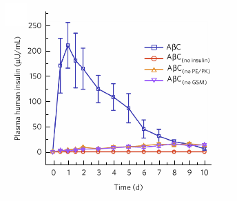
To test how their system actually responds in a biological medium, the authors apply a gel under the skin of mice that contains the OLVs. For a group of diabetic mice, this artificial beta cell system showed a significant effect on the measured insulin levels in the mice blood. For control groups; (i) with no insulin ($latex A \beta C_{no insulin}$), (ii) with no lipid fusion system $latex A \beta C_{PK/PE}$ (PK and PE are DNA molecules that mediate the fusion process), and (iii) with no glucose sensing machinery $latex A \beta C_{no GSM}$, the insulin release was minor over the course of 10 days (see Figure 2). But when the insulin-loaded artificial cells were administered, the mice’s insulin levels increased remarkably over the control cases.
All in all, Chen and colleagues manage to release insulin in a controlled manner. There’s no need to evade an organism’s immune system–the OLVs don’t provoke an immune response. There’s also no need to inject insulin–it’s released automatically when needed. This work gives hope of drastically improving the lives of the nearly half a billion people worldwide suffering from diabetes.
[1] You might be asking: why do pancreatic cells secrete a polymeric form of sugar in response to low blood sugar level?! Well, which one is faster and more effective to you? Releasing one-by-one a single sugar, or releasing one-by-one a bag full of sugar molecules (the polymeric form). When this polymer leaves the cell quickly, it bursts (dissociates) into single sugar molecules, later to be absorbed by relevant cells.
[2] Under some circumstances that might be due to genetics, the body’s immune system attacks the beta cells and destroys them. These are called autoimmune disorders.
[3] Glucose oxidase (GOx) and catalase (CAT) are working in parallel to transform the glucose signal into protons. GOx, with the help of an oxygen molecule, converts the glucose to gluconic acid releasing a proton. But there is a by-product of this reaction which is not favored. The hydrogen peroxide ($latex H_{2}O_{2}$) produced is very active that can mess up all the molecules inside the giant vesicles. With a nice trick, the researchers simultaneously convert the hydrogen peroxide to oxygen by adding CAT enzyme. Now, this is feeding two birds with one seed. Getting rid of ($latex H_{2}O_{2}$) while providing the oxygen for the GOx to do its job.