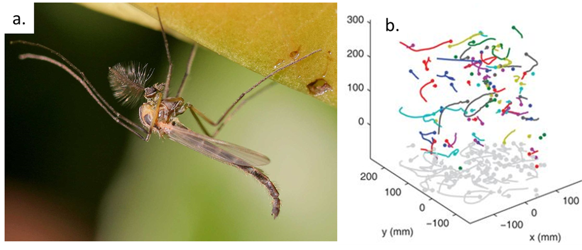
Imagine yourself as a small fly called a midge (shown in Figure 1a). You used to live in a lake as a small larva with no concerns in life except swimming, eating, and growing. One day, you hid underwater and formed a cocoon around your body as it developed wings, legs, and antennae. A few days later, you swam to the surface and burst out of your cocoon as an adult fly — a male. As a new adult male, you find the clock ticking – you have only a few days to find a mate before you die.
Attracting a female is difficult for a tiny midge – how is she going to see you flying around? Fortunately, you can team up with hundreds of other male midges. Together, you fly above the lake in a stationary swarm that looks like a large cloud. Females can find this swarm and fly into it for their choice of mate.
In today’s study, Douglas Kelley and Nicholas Ouellette investigate how the motion of midges in a swarm helps the swarm stick together.
Figure 1. (a) A midge is a tiny fly that forms mating swarms above lakes (image from Wikipedia). (b) Midges tracked in a swarm in the laboratory, with different midges in different colors (Figure adapted from original article)
The researchers set up midge swarms in the laboratory and film them with three infrared cameras. They track all of the individual midges in the swarm and calculate their trajectories. Tracking dozens of small midges is not easy! First, they use the 2D images from the three cameras to locate the flies in 3D for each frame. Then, they use a technique originally developed for studying turbulent fluid flows to generate the trajectories over time. This technique uses the history of each midge to estimate where it is likely to be next and looks for midges in that area at the next time step. The resulting trajectories are shown in Figure 1b. The positions, velocities, and accelerations of the midges give clues about how the swarm moves.
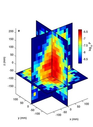
First, Kelley and Ouellette discuss the position of the midges. They plot the logarithm of the probability ($latex log_{10} P$) of finding a midge in a point in the swarm in three dimensions in Figure 2. Bright red represents a high probability of finding a midge, and blue represents a very low probability. Midge swarms are nearly symmetric, but larger swarms (of 100 individuals or more) are slightly taller than they are wide. This is unlike bird flocks, which are nearly two-dimensional.
Figure 2. Probability of finding a midge at x, y, and z coordinates in the swarm. Bright red colors indicate high likelihood of finding a midge, and blue represents a very low chance of finding a midge in that position. (Figure adapted from original article)
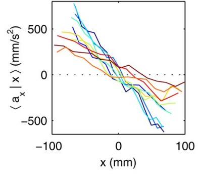
The researchers then investigate the velocities of the midges. Since the swarm is stationary, the average velocity of all the midges in the swarm is nearly zero. It turns out that the standard deviation, or the variation, of the velocities of the individual midges is more useful for understanding the motion inside the swarm. Midges fly twice as fast horizontally as vertically, just like birds in a flock. However, unlike flocks of birds, the midge swarms are not polarized — a midge does not tend to fly in the same direction as its neighbors. Finally, Kelley and Ouellette investigate the acceleration of the midges in the swarm. The midges are equally likely to turn in any direction, unlike birds or fish. Relative to their body size, larger animals have more inertia than smaller ones, and must exert a lot more effort to turn, accelerate, and decelerate. Thus, they tend to keep moving in the direction they are currently moving. Midges, on the other hand, can turn and easily move in any direction. Kelley and Ouellette find the average acceleration of the midges in the swarm in the x-direction as a function of the midge’s x-position, $latex \langle a_x|x \rangle$, in Figure 3. The midges tend to accelerate towards the center of the swarm, keeping the entire swarm together despite the midges’ constant motion. [1]
Figure 3. Acceleration of the midges in the x-direction as a function of the x-position for several midge swarms. Each line represents a different swarm. When a midge is at the right edge of the swarm, it accelerates to the left (and vice versa). (Figure adapted from original article)
In this study, Kelley and Ouellette quantify a new type of swarming behavior. Unlike most other animal aggregations like bird flocks and fish schools, midge swarms stay in one place, helping female midges find the love of their very short lives.
[1] Surprisingly, when Kelley and Ouellette investigated the mean square displacement of the midges, they found that the midges act as if they are trapped in a box with walls.
If we could shrink a submarine down to the microscopic scale, could we pilot it into the human body to fight infection and perform surgery? Despite suggestions from futuristic sci-fi such as “Fantastic Voyage”, “Honey, I Shrunk the Kids”, “The Magic School Bus”, “Power Rangers”, and “Rick and Morty”, we cannot survive such shrinking and our vessel would be without a pilot. But it may still be possible to “shrink” down some of our technology and control it remotely as we will see from researchers at MIT in this week’s paper.
Intheir letter to Nature, author Yoonho Kim and colleagues at the Zhao lab reveal a dazzling zoo of tiny transformable machines. Following recent trends in the metamaterials community, they built a series of “origami” and “kirigami” samples inspired by the cutting and folding of traditional Japanese paper art.
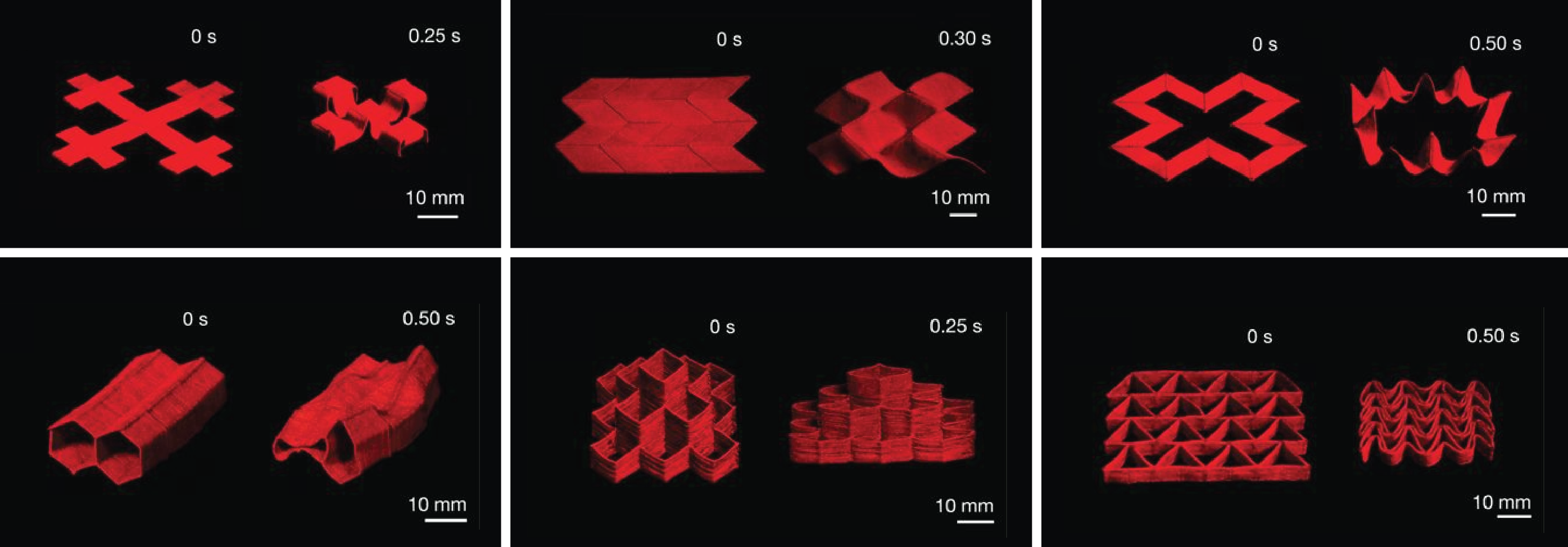
But, unlike traditional origami, these special sheet-like materials are able to fold themselves up and change shape on command, as shown in Figure 1. With this remarkable new technique, they assemble panels and tubes into a variety of structures which can shrink, shear, expand, and change shape, as well as pipes which can obstruct themselves on command.
Figure 1. Microstructures made from thin, flexible magnetic panels fold and reshape themselves on command in less than 1 second.
To create these machines, Kim combines two relatively simple ingredients: 3D printing and magnets. These tiny gadgets do not resemble conventional robots and are better described as 3D printed flexible materials with specialized ferromagnetic regions. So let’s break these ingredients down piece-by-piece.
The process of 3D printing involves a nozzle depositing an “ink”. As the ink leaves the nozzle, it sticks and transitions from a fluid state to a hard or rubbery state, becoming a solid piece of the “printout”. By choosing where to put these squirts of ink, a 3D printer is able to quickly and accurately build 3D structures.
Typically this ink is some sort of molten plastic or rubber, but by including tiny magnetic bits in the ink and applying a magnetic field as it passes through the nozzle, the magnetic bits will reorient themselves and the ink can adopt the magnetic properties of the applied field. Then, as the ink hardens, this magnetic alignment will be “frozen in”. The result is a flexible material that “remembers” the magnetic field that was present when it formed. And what’s more, by changing the direction of the applied magnetic field over the course of printing, the material can be programmed with regions of different magnetic orientations.
Now, when this printed and patterned material is exposed to a magnetic field again, all these little magnetic regions of the material will try to align themselves with the field. The result is a controlled and predictable change of shape. Careful design of these magnetic domains by Kim and colleagues is the secret behind their self-folding origami as well as complex shrinking and reshaping materials, which seem to be just the tip of the iceberg.
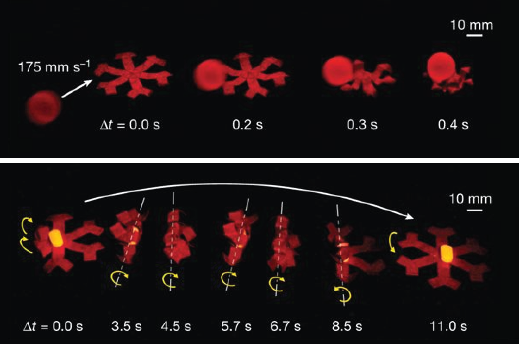
Figure 2. Controlled by an external magnetic field, a “soft robot” displays dual functionality by catching a fast moving object (top) and rolling a wrapped load across a distance (bottom).
While all these machines are controlled remotely, the material design is permanent and raises questions of multifunctionality. As an inspiring counterexample, the researchers present a flat “soft robot” which can crawl, catch, and can even wrap and roll a small load across a distance as shown in Figure 2. The variety of moves available to this robot stem from clever dynamic variations of the external magnetic field. To really appreciate all of these devices, be sure to check out the videos in theSupplementary Section in the paper (definitely don’t miss Video 8).
Perhaps these dynamic contraptions could soon be deployed inside a living creature, opening the door to new surgical and diagnostic techniques. While an individual robot may be limited to some simple pre-designed action, many medical applications like cutting and sewing are simply repetitive, basic movements. While this possibility has inspired many researchers in the Soft Matter community and beyond to start building a remarkable variety of tiny robots, none of them have yet found their way into the human body to complete a medical task.
In medical applications, biocompatibility is crucial, for both the object itself and its control mechanism. Fortunately, the magnetic fields used in this research can be safely applied to a human body — the field strengths used in Zhao’s lab are lower than those in standard MRIs. However, these robots currently occupy a size scale of roughly 1 centimeter across – HUGE in biological terms. To perform non-invasive surgery, a robot would need to shrink down closer to the micron scale. So it appears that the future of this game will be akin to the development of the transistor: a search for the small and the powerful.
If you just landed on Softbites for the first time, you probably have not had the chance to read our previous posts about microfluidics (like this one, or that one, and more). If this field of science is foreign to you, all you need to know is that it studies how fluids flow at really small scales (typically tens to hundreds of micrometers). For instance, you can quickly generate tiny droplets of a solution, turning each droplet into an individual “reactor”. Or you can create microenvironments with precisely controlled chemical concentrations to grow cells in different conditions.
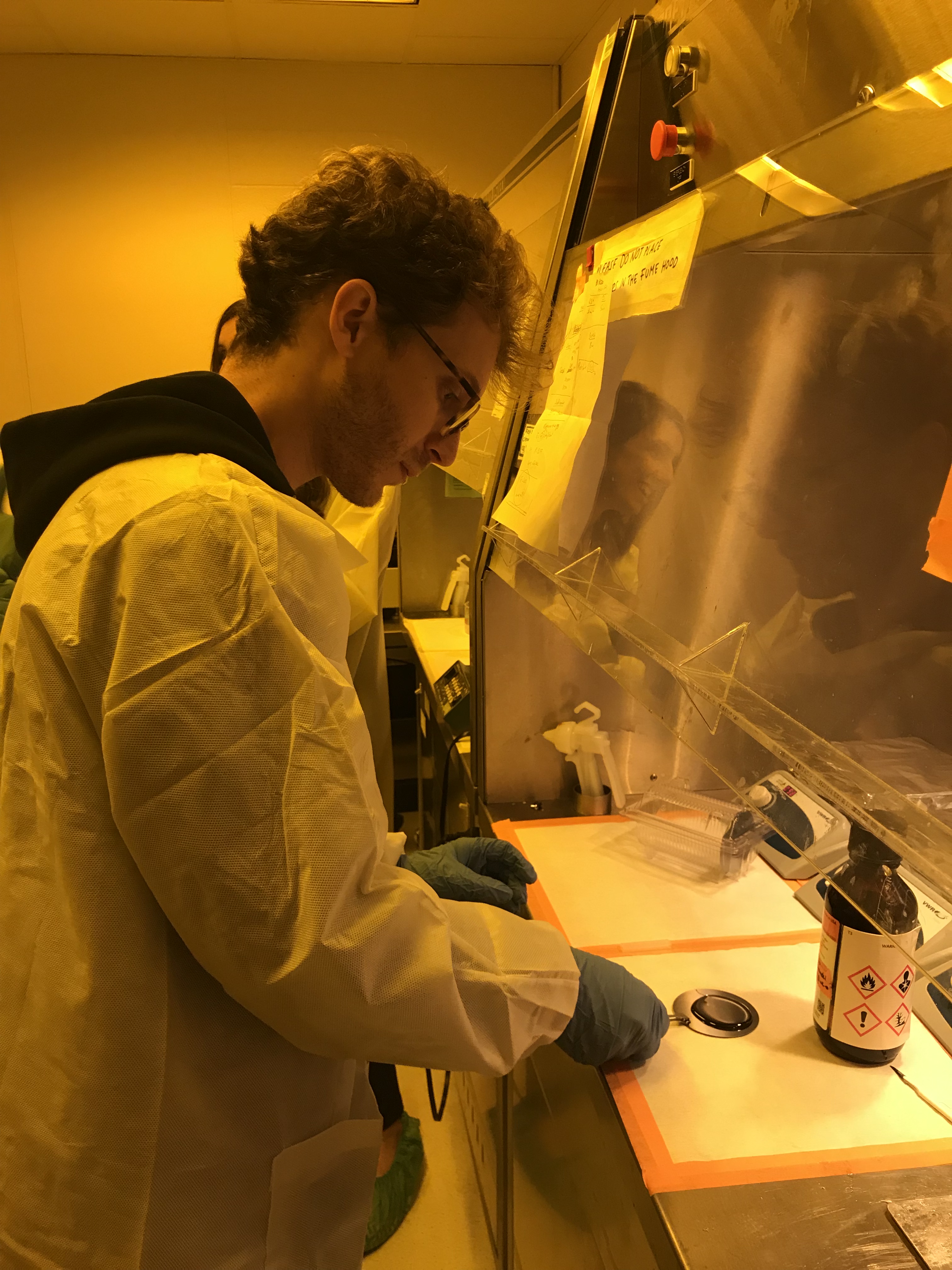
In addition to being a thriving field of research, I think microfluidics is simply beautiful! I have spent hours looking at the Softbites website’s banner, a movie of droplets that was shot by the Lutetium project. You can imagine my excitement when I registered to the annual MRSEC microfluidics summer course 2019 at Brandeis University. This summer course was run by four talented grad students from the Fraden lab and the Rogers lab: Ali Aghvami, Alex Hensley, Marilena Moustaka and Zahra Zarei. These labs are part of the MRSEC program at Brandeis, an important place in the New England soft matter community. Therefore, I think it was the perfect place to get started with microfluidics!
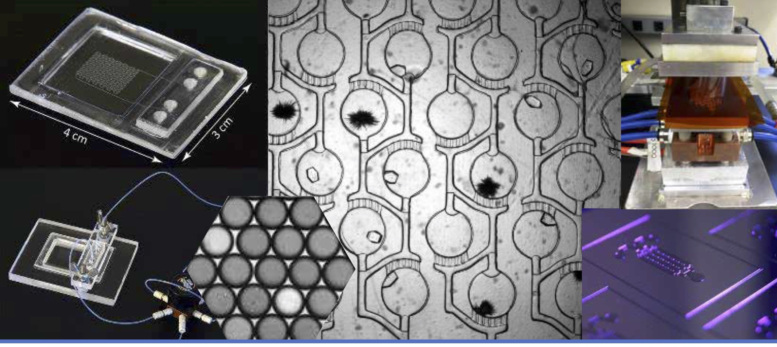
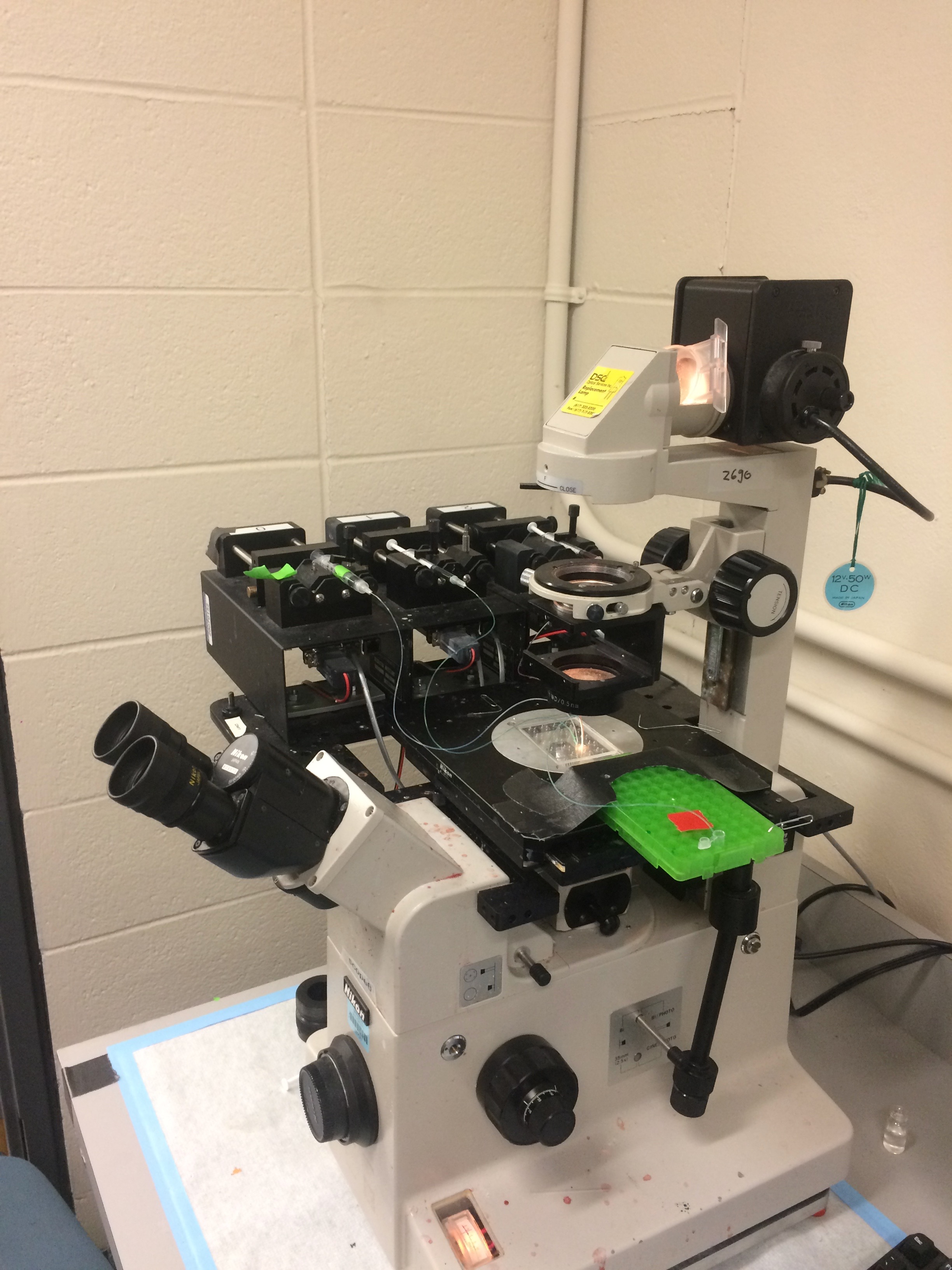
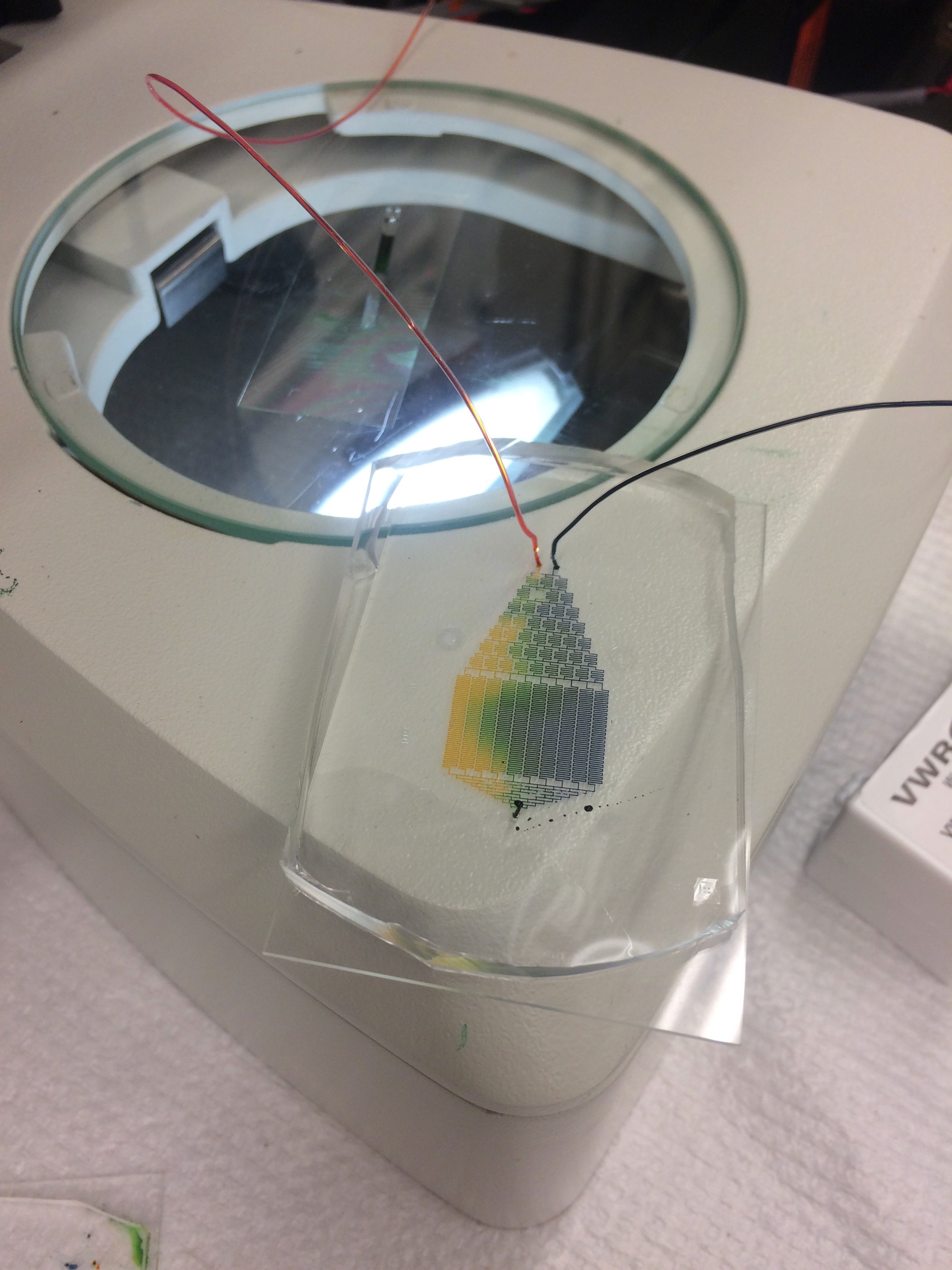
Figure 1. Me, trying to pour some resin on a silicon wafer (left). A drop maker setup (middle). A gradient maker chip, with a defect leading to a non-stable gradient (right).
Over five days, we learned the basics of one of the standard methods for making microfluidic channels, called soft lithography. The rationale is to make a mold using a UV-light sensitive resin. A 2D pattern can then be polymerized in the resin by shining UV-light through a mask. Whatever the UV light hits gets hard, while the rest of the resin stays soft. The soft resin is washed away leaving only the hard, UV-treated resin behind in the shape of the mask. The mold will finally be used to imprint the design in a soft transparent material called PDMS (a very nice video from the Lutetium project explains all this process). We experimented with this fabrication during three main sessions:
We drew our 2D design using a drawing software
We fabricated our mold in a clean room so no dust ruined our tiny features
We cast the PDMS on the mold and sealed the device with a glass slide
We were taught each of these steps through a combination of lectures and hands-on sessions. You can see a droplet maker and a gradient making device that we made in Figure 1.
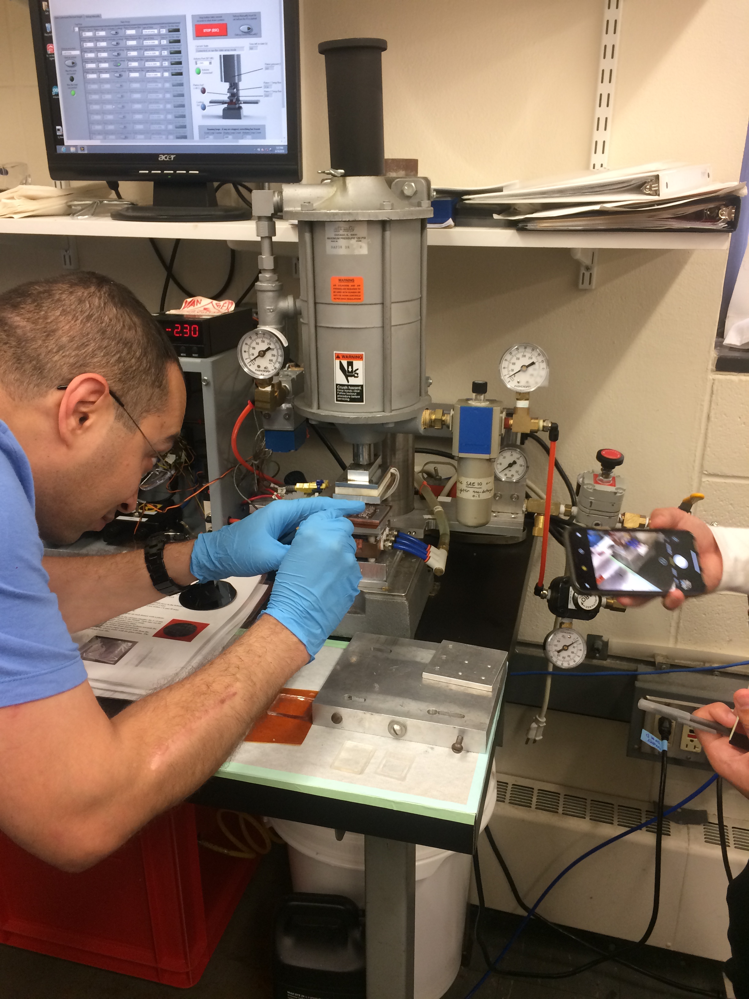
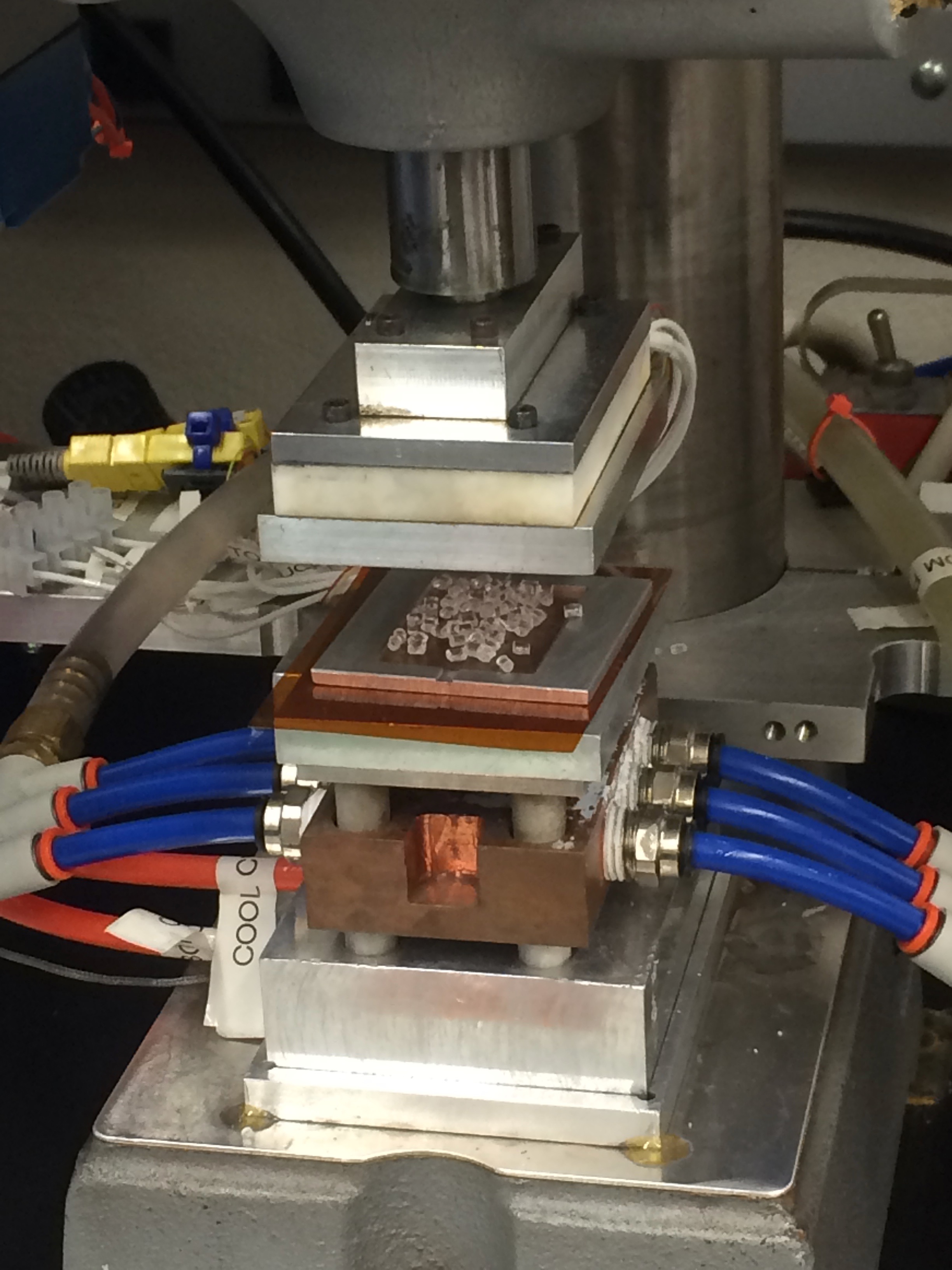
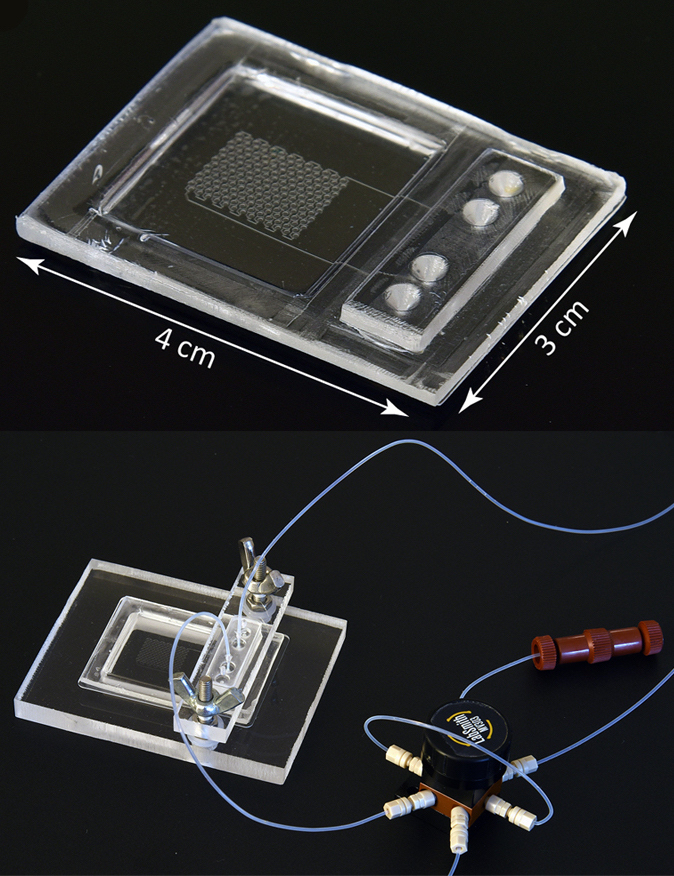
In addition to learning how to make these routinely used PDMS-based devices, we were also introduced to another technique used in the Fraden lab. This technique, which was recently published (2017), uses a thermoplastic (a plastic that melts at moderate temperatures) as the main device material. This thermoplastic can be cast onto a PDMS mold by means of a thermopress (as shown in Figure 2). Unlike PDMS, thermoplastic is not permeable to water and organic solvent, and is stiffer. If the permeability of PDMS is a limitation for your microfluidics application, thermoplastic might be the way to go!
Figure 2. Ali Aghvami placing thermoplastic chips onto the PDMS mold (left). Close-up on the thermoplastic in the thermopress before being cast (middle). The final device (right), from Aghvami et al. 2017.
This week-long course introduced us to both classical microfluidics techniques that are routinely used in labs and some more advanced ones. More importantly, our instructors dedicated important time to discuss our personal projects with us. We even had a consulting session with Seth Fraden! I strongly encourage anyone to attend the next editions of this course. Each year, the dates and the call for applications are released in spring, so don’t miss out!
These were my first drops! I literally spent 45 minutes watching them!
Many consumer products, such as clothes and food packaging, are made of blends of polymers, long molecules consisting of repeating chemical units. The attractiveness of using blends of different polymers arises from the engineers’ desire to combine multiple unique properties of each individual polymer, such as transparency, stretchability, and breathability, into a seamless whole. However, different polymers are not necessarily miscible, a term scientists use to describe whether two materials mix at the molecular level. Miscibility isn’t a one-and-done kind of deal: scientists and engineers have known for years how to make polymer blends mix by careful temperature control. What if there were conditions other than temperature to achieve polymer blend miscibility? This may ultimately help in industrial processing of polymer blends. In this week’s paper, Professors Annika Kriisa and Connie B. Roth from Emory University in Atlanta, Georgia, explore the mixing dynamics of two polymers by using a strong electric field.
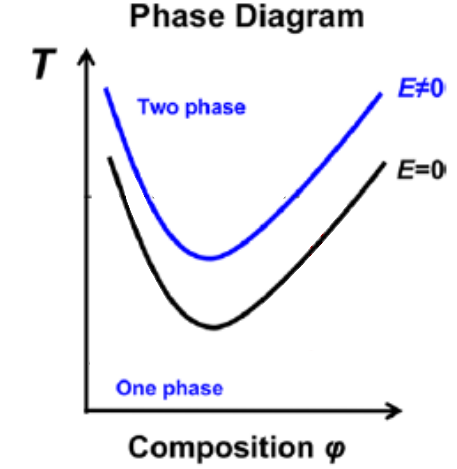
Figure 1. Miscibility diagram of a hypothetical polymer blend consisting of polymers A and B. The x-axis is the fraction of polymer A in the blend (Composition ?) and the y-axis is the temperature of the blend (T). The curves represent the temperature above which the blends are immiscible without an electric field (black curve) and with an applied electric field (blue curve). The presence of the electric field increases the miscibility of the blend (higher transition temperature) at a given fraction of polymer A. (Image adapted from original paper.)
Before we dive into the meat of the paper, it’s important to know how temperature affects the miscibility of a polymer blend. The black curve in Figure 1 is a representative miscibility diagram of two blended polymers, which shows the temperature at which a polymer blend transitions from being miscible (below the black curve) to immiscible (above the black curve) as a function of the fraction of one polymer (denoted Composition ?) of the blend itself. The polymer blend is considered more miscible if the miscibility curve is shifted upwards, so that the blend turns immiscible at a higher temperature (see blue curve in Figure 1).
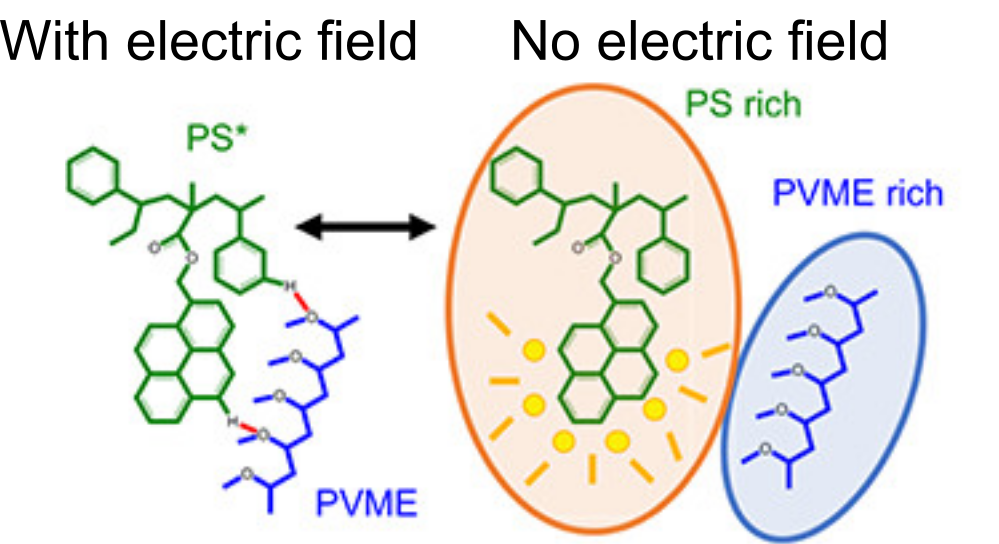
Kriisa and Roth wanted to explore how the application of an electric field influences the mixing dynamics of polystyrene (PS) and poly(vinyl methyl ether) (PVME) polymers. You may be quite familiar with these materials: PS is the formal name of styrofoam, the main component in plastic cups, and PVME is typically used in glues and adhesives. In the past, Kriisa and Roth studied the effect of electric fields in blends of these materials, and found that the electric field enhances polymer blend miscibility: an electric field raises the temperature at which a PS/PVME blend becomes immiscible, similarly to the blue curve in Figure 1 [1]. What interested the authors the most in this today’s paper was the dynamics of mixing; in other words, how quickly do immiscible blends remix once they are exposed to an electric field? And what can we learn about the factors governing the remixing process?
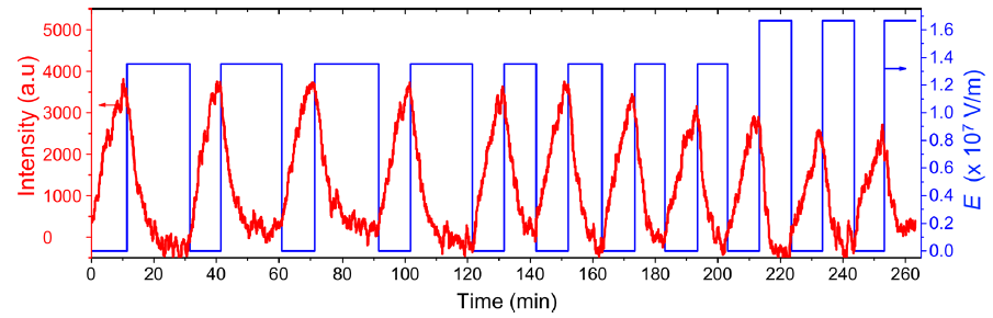
Figure 2. Switching the miscibility of polystyrene/polyvinyl ethyl ether (PS/PVME) polymer blends as a function of time through the application of an electric field (E). The red curve is the intensity of the fluorescence of a molecule attached to polystyrene, which decreases with time. The blue curve is the imposed electric field, which is repeatedly switched on and off. (Image adapted from original paper.)
The authors showed that the dynamics of mixing a PS/PVME blend is highly sensitive to the application of an electric field. They demonstrated this by examining a PS/PVME blend at the temperature four Kelvin higher than the temperature at which it becomes immiscible. They repeatedly switched on and off an electric field regularly, causing the blend to switch from being miscible to immiscible (see blue curve in Figure 2). To determine how well mixed the blend was, they measured the intensity of the light emitted by a fluorescing molecule, which was chemically attached to the PS molecules (see red curve in Figure 2). When PS and PVME are fully mixed, the fluorescence intensity decreases to 0. After switching on the electric field, the blend starts mixing immediately, showing a high sensitivity to the presence of the electric field.
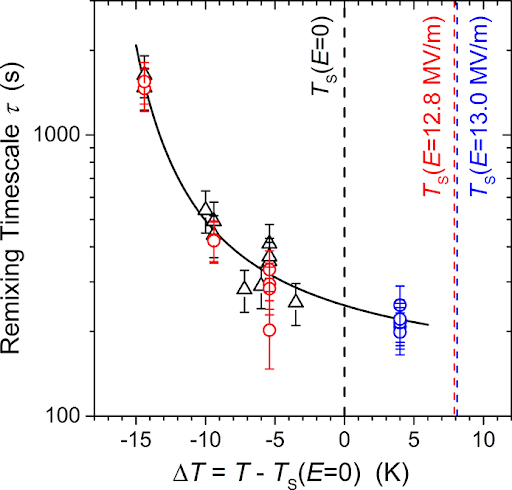
Figure 3. Remixing timescale (?) as a function of temperature (T) and applied electric field (E). The black symbols correspond to absence of electric field, red to electric field at E =12.8 MV/m, and blue at E=13.0 MV/m. Ts (shown by the dashed lines) is the temperature at which the blend becomes immiscible at the given electric field. The remixing timescales follow the same black curve, showing that they are largely independent of E. (Adapted from original paper.)
The authors repeated this experiment for a variety of temperatures and electric field strengths. From the fluorescence curves, they extracted the remixing timescale or the time it takes for the blend to remix, as shown in Figure 3. The black symbols correspond to absence of electric field, while the red correspond to E = 12.8 MV/m and the blue to 13.0 MV/m. One may notice that the time it takes for the polymer blend to remix is largely independent of the electric field strength at a given temperature, since all remixing timescales (?) follow the same black curve. Thus, the authors concluded that the rate of remixing is not affected by the electric field.
In short, Kriisa and Roth showed that the dynamics of remixing polymer blends are sensitive to electricity. They found that immiscible blends immediately begin to remix when exposed to an electric field and that the time it takes for the blend to completely remix is independent of the field’s strength. From an industrial perspective, this shows that the miscibility of polymer blends can be influenced by factors other than temperature. An important advantage is that an electric field can be applied uniformly and instantaneously, whereas changes in temperature take time to propagate through materials. Thus, engineers may be able to instantly tune the miscibility of polymer blends using electric fields; a discovery that may lead to future technological advances in devices and materials whose properties would be quickly ‘’switched’’ through electricity.
When an experiment doesn’t behave the way we expect, either our understanding of the relevant physics is flawed, or the phenomenon is more complicated than it appears. When a theoretical prediction is off by two orders of magnitude – like what was observed in this recent paper by Hua Yung Lo, Yuan Liu, and Lei Xu of the Chinese University of Hong Kong – something is seriously wrong.
If Lo and colleagues drop a liquid droplet onto a smooth, flat surface, it will take on an equilibrium shape which depends on the properties of the liquid and solid materials at the interface (eg. water on Teflon will form a nearly perfect spherical drop while water on stainless steel will spread out, forming a spherical cap). For low viscosity fluids, the equilibration process happens almost instantly… unless the surface is very flat and very smooth.
If the surface below a droplet is atomically smooth (not a single atom is out of place to roughen the surface), a thin layer of air will form between the droplet and the surface, keeping the droplet from making contact with the surface. Eventually the trapped air will escape, draining out like how a liquid would, allowing the droplet to collapse onto the surface. Traditional fluid dynamics simulations predict that the collapse would take between 10 – 100 seconds. In experiments, however, contact generally happens in less than one second. Lo and coworkers set about investigating this seeming contradiction by observing the flow that happens within the air and liquid at the boundary between a droplet and a smooth surface.
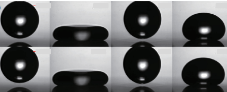
To study this problem, the researchers dropped small spherical oil droplets (1.7 mm diameter) onto a glass surface with a very thin coating of oil which could be tilted. They observed that droplets would compress and bounce as they floated on a pocket of air, before collapsing onto the surface. The contact area was imaged from the bottom and side simultaneously using two high-speed cameras. Side-on sequences are shown in Figure 1 with a slightly tilted surface (a) and a perfectly leveled surface (b). While both droplets collapsed onto the surface far quicker than predicted by simulations, the droplet on the leveled surface was observed to float just above the surface approximately 10 times longer than on the tilted surface before collapsing.
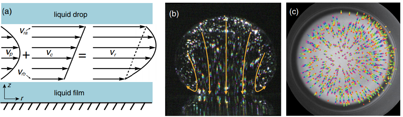
Figure 1. A time sequence of an oil droplet being dropped on an atomically smooth, oil coated, glass surface which is a) slightly tilted (0.3°) and b) leveled (0°). c). Schematic of the droplet and surface. A video of the process can be found here (Figure adapted from the original paper.)
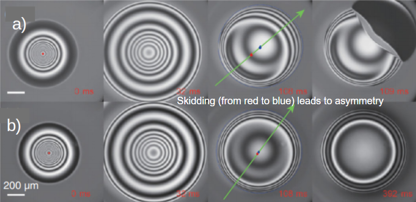
The effect the tilted surface has on this phenomenon became more apparent when viewed from below. On the tilted surface, the droplet would “skid”, observed as a sliding of the droplet’s center from the red point to the blue point in the direction of the green arrow as shown in Figure 2 a) while the size and shape of the air pocket was measured using two-wavelength interferometry [1]. Tilting the surface caused an asymmetric air pocket to develop, with a thinner gap at the front of the droplet and a thicker gap at the back. When a droplet did not skid, it formed a symmetric air pocket like in Figure 2 b). A thinner gap (with difference of just half micrometer) lets the air drain out (and allows contact to be made) much faster than it would for a symmetric air pocket on a flat surface. However, even a flat surface drained 10-times faster than expected.
Figure 2. Images of the bottom of an oil droplet coming in contact with an oil-coated glass slide that is a) slightly tilted, showing a droplet skidding until it reaches full contact with the surface at 109 ms, and b) perfectly leveled, where the droplet still has not contacted the surface at 392 ms. Light and dark bands correspond to the change in thickness of the air pocket. A video of the process in a) and b) can be found here and here.
To understand the flow of air from under the droplet, the researchers modeled it as a low-viscosity fluid. When a low-viscosity fluid flows past a wall (like water through a tube), the friction at the walls may reduce the flow near the walls to something-close-to-zero. This is called a “no-slip boundary condition”. On the other hand, a “plug flow boundary condition” means there is significant slip and therefore flow along the walls. Each of these boundary conditions lead to characteristic velocity profiles like those presented in Figure 3 a). Typically, one would assume that air flowing through the air pocket near the oil interface would have a no-slip boundary condition while something like a sludge or gel would demonstrate plug flow. Yet, it is this assumption that ends up being incorrect.
The researchers measured the velocity of oil within the oil droplet and the surface coating using particle image velocimetry, a technique where small light-reflecting particles are mixed into a material and tracked down as they move along with the surrounding fluid. An image of the oil droplet seeded with the tracer particles is shown in Figure 3. In this way, the researchers were able to directly visualize flow of oil at the air-oil boundaries, finding a sort of “slip layer” along the walls corresponding to the layer of oil being dragged along by the air. This lets larger volumes of air drain from under the droplet, explaining the surprisingly short time it takes for droplets to collapse onto the surface.
Figure 3. a) The velocity profile of air under the droplet (Vr) is a combination of a no-slip (Vp), and slip (Vc) boundary conditions. b) Side-view image of an oil droplet. White dots are reflective particles with velocity shown as yellow arrows. c) Bottom-view of the same oil droplet where the colored streaks (red to purple) trace the flow of the oil on the surface. (Figure adapted from the original paper.)
Despite its apparent simplicity, Lo et al. revealed a fundamental misunderstanding in the way scientists thought about how fluids flow near an interface. Accounting for the effect of slip, the researchers unified both theory and observation and explain why liquid droplets will make contact with a perfectly smooth surface so much faster than originally expected.
[1] a technique that uses light interference to quantify changes in thickness as light and dark bands; narrow bands correspond to rapidly changing thicknesses, much like the lines on a topographic map show changes in elevation. ^
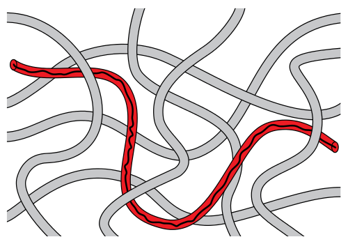
Scientists often draw inspiration from biological organisms to describe phenomena, even when they are studying outside the realm of biology. Physicist Pierre-Gilles de Gennes[1] was no exception. In 1971, after being inspired by the movement of snakes, he proposed reptation theory, or the reptation model, which has since been widely used to describe motions of polymers[2]. As the name “reptation” suggests, de Gennes assumed polymer chains move like snakes. As shown in Figure 1, the model describes a polymer chain’s motion in an environment that is highly populated by other chains (shown in gray) by assuming that the chain is confined in a virtual tube (shown in red) formed by surrounding polymer chains. According to reptation theory, the chain wiggles through this tube, similar to a snake slithering through the woods. As one might imagine, directly imaging the snake-like slithering of polymers is a challenging affair; however, in today’s study, Maram Abadi and coworkers from King Abdullah University of Science and Technology were able to do just that with DNA chains – an example of a polymer – and compared their results to prevailing theory.
Figure 1. A schematic of the reptation model. In a crowded and entangled polymer environment, a long and linear polymer chain (black) is located in a virtual tube (red), which traces the chain trajectory. Surrounding polymers are shown in gray. (Adapted from the Wikipedia page for reptation.)
While reptation theory has done fairly well in describing experimental observations of polymers, there are some shortcomings to both the experiments supporting this theory as well as to the theory itself. Namely, previous experiments mostly considered the overall motion of the chain; but local chain motion, such as motion at the ends of a polymer chain, have not been thoroughly studied. In addition, the theory was only designed for polymers with two ends, known as linear polymers. Thus, it does not account for the dynamics of polymers with different geometries, such as those that form rings, known as cyclic polymers. Given these observations, Abadi and coworkers realized that there was more work to be done in the studies of polymer dynamics.
To scrutinize the movements of the polymer chains, the authors used super-resolution fluorescence localization microscopy[3], which lets them monitor the movements beyond the typical microscopy resolution of ~200 nm. This technique allowed Abadi and coworkers to not only observe whole-chain dynamics but also local dynamics. To test the predictions of reptation theory, they chose both linear and cyclic DNAs with fluorescent dyes attached as model polymers for their study.
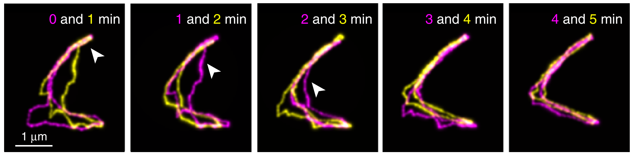
Figure 2. Fluorescent images of a linear DNA chain collected at different time points (indicated in the figure), overlapped for comparison. Insets show the enlarged views of the highlighted areas. (Adapted from the original paper.)
First, linear DNAs were used to confirm what has been known from reptation theory in great detail. Shown above in Figure 2 are images of a linear DNA as a function of time. Their results were consistent with theory. First, polymer chains traveled along virtual tubes that followed the contour of the chain (shown in white boxes in Figure 2A). Second, most of the polymer chain’s displacements were within the confinements of the virtual tubes, which had a diameter around 51–95 nm (shown in red boxes in Figure 2B). Further, they occasionally saw displacements of the DNA that exceeded the size of tube diameter (shown in cyan boxes in Figure 2C), known as constraint release in reptation theory. Finally, Abadi and coworkers observed that the chain-ends were able to move farther than the centers of the chains, which in turn creates a new tube for further DNA reptation (shown in green boxes in figure 2C). In reptation theory, this is called contour-length fluctuation.
However, there was one particular deviation from the theory found in the authors’ results. While the chain-ends were expected to move more freely than other parts of the chains, the chain-end motions were a lot faster than what is predicted by reptation theory. Therefore, the authors concluded that the motions at the chain-ends were beyond the scope of the reptation theory. These unexpectedly fast movements were not observed in previous experiments, in which only the chain as a whole was considered.
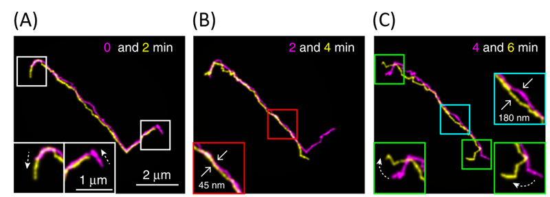
Figure 3. Both rows are fluorescent images of cyclic DNAs collected at different time points (indicated in the figure), overlapped for comparison. 3A shows amoeba-like motion, and 3B shows contracting of an open structure. More details can be found in the main text below. (Adapted from the original paper.)
The authors also observed cyclic DNAs using the same methods. As they are not linear, reptation theory fails to accurately explain their movements. The authors observed diverse motion of the cyclic DNAs. You may notice in Figure 3A that the cyclic DNA has a loop-like region, shown in the white boxes. They found that cyclic DNAs repeatedly contract and extend this region, resembling the motions of amoeba. In addition, as shown in the first panel of Figure 3B, some cyclic DNA molecules may start with an open structure. However, as time progresses, these open DNAs may contract into more linear forms and expand back into the open shape again. Thus, Abadi and coworkers were able to show two phenomena that cannot be explained by reptation theory, thus requiring it to be further refined.
The results of this paper support many of the conclusions of reptation theory; however, it does suggest that there is still a need to expand this otherwise well-accepted theory. By considering different geometries and shorter timescales, this theory will be more powerful as a predictor or explainer of novel polymeric material dynamics. Furthering the understanding of polymer dynamics will then help us understand polymer properties for use in a variety of applications that we see in our lives every single day.
[2] Polymers are molecules that are consist of repeating chemical structures.
[3] Super-resolution microscopy is a technique that lets us observe things that are smaller than the diffraction limit of ~200 nm, which is the limit that is imposed by the physics of light.
If you ever played tug-of-war in elementary school, you might remember that it isn’t the friendliest game. People fall over, hands get burned from holding on to the rope, and knees get scraped from falling on the ground. Although victory can be sweet, the injuries that come with it may make you never want to play the game again. Perhaps surprisingly, there is a similar ‘’tug-of-war” happening inside your body, as individual cells move around from one place to another in a process called cell migration. What’s more, this microscopic tug-of-war may help to heal those scrapes and bruises that happened in elementary school, and those that happen in your everyday life.
A single cell moves by detaching and reattaching from the substrate, or the surface it is on, as the cell expands and contracts. This movement exerts forces on the substrate. (These forces can actually be measured directly – this is the topic of a previous softbites post.) When many cells move together in a “cell sheet”, their motion becomes more complicated. Not only do cells push and pull on the substrate, but they also push and pull on the cells that surround them. In today’s study, Xavier Trepat and colleagues show that there is a “tug-of-war” between cells that causes them to migrate.
Previously, it was thought that only the cells at the very front of the mass of migrating cell, or the leading edge of the cell sheet, exert forces on the substrate. According to this picture, most of the cells get passively pulled along by the leading edge, and neither push nor pull on the substrate. By measuring the forces the cells exert on the substrate, Trepat and his colleagues discovered that, in fact, all of the cells are involved in pushing the cell sheet forward.
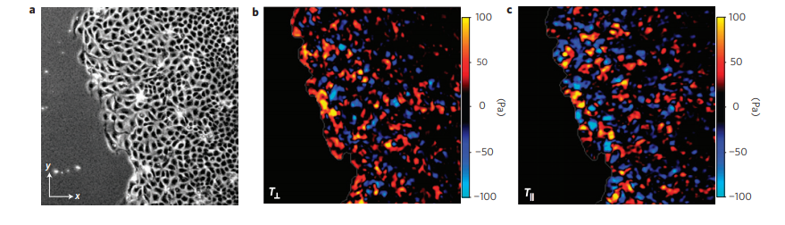
The researchers measured the forces in a moving sheet of cells, taken from canine kidneys, growing on a gel substrate using a technique called traction force microscopy. The first step of this technique is to track the displacements of different points within the substrate as the cells move. Then, the mechanical properties of the gel are used to calculate the forces on the substrate generated by this motion. The researchers mapped the value of these forces using different colors, with red and blue representing very strong forces and black representing zero force. They first looked at what happened at the leading edge of the cell sheet, as in Figure 1.
Figure 1. a. Image of the cell sheet, in which individual cells are outlined in white. The field of view is 700 microns by 700 microns. b. The forces that the cells exert perpendicular to the leading edge of the cell sheet. c. The forces that the cells exert parallel to the edge of the cell sheet. Bright red and blue colors indicate strong forces (up to 100 Pa of stress), while black color indicates low forces. (Images adapted from the original article.) The cell sheet’s expansion was recorded in a video as well.
The researchers separated the normal forces (Figure 1b) — those exerted by the cells perpendicular to the leading edge of the cell sheet, or in the direction of the cells’ motion — from the forces exerted parallel to the leading edge of the cell sheet (Figure 1c). The bright red and blue colors in Figure 1 show that cells well inside the cell sheet exert forces on the substrate. From this, they hypothesized that instead of having “follower” and “leader” cells, all the cells contribute into pushing and pulling the cell sheet as they move.
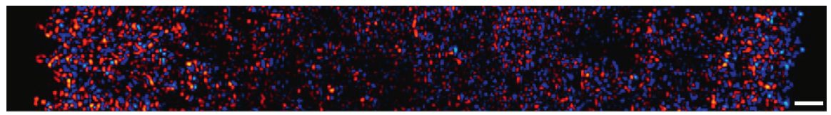
The researchers then looked at larger areas of the cell sheet, such as that shown in Figure 2. The bright colors near the edges correspond to strong forces, while the black spots show that the forces in the center of the cell sheet are weaker. This suggests that the cell sheet “tugs” both to the right and the left as it expands. As the cells exert forces on the substrate, they exert forces on each other. The cells pulling to the right and the left are similar to two teams pulling a rope in a game of tug of war. The sheet of cells is like a rope that grows in the direction of the tugging of the cells.
Figure 2. Forces exerted by a larger piece of the cell sheet. Bright red indicates strong positive forces and blue indicates strong negative forces, while black indicates low forces. The scale bar on the bottom right is 200 micrometers. (Image adapted from the original article.)
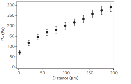
Next, the researchers wanted to understand how being tugged on by its neighbors affects the motion of individual cells: does the tug of war consistently pull a cell in a particular direction? Or is the cell equally likely to be pulled in any direction? To answer this question, Trepat and colleagues measured the average force exerted on a cell by its neighbors, as a function of the distance of that cell from the edge of the sheet. If each cell was moving independently, the average normal force inside the sheet would be zero – on average, no cell would be pushing or pulling any other cell to a specific direction. Instead, as shown in Figure 3, the average force was not zero, and was actually higher for distances farther from the sheet’s leading edge. In other words, the cell sheet is expanding from the inside more than it’s being pulled from the edge.
Figure 3. The average normal force exerted on a cell by its neighbors, $latex \sigma_{xx}$, is higher farther from the leading edge of the cell sheet. (Figure adapted from the original article.)
Each individual cell crawling on a substrate has little effect on its surroundings, but many cells acting together can exert forces on each other to guide the collective in a particular direction. As cells replicate, such as in a healing wound, this guiding helps the cells expand in directions where there is space to be filled. This study by Trepat and colleagues reveals for the first time the tug-of-war that allows the tissues in our bodies to grow and heal.
It’s unusual to run a symposium as a PhD student, but anyone can do it! I was lucky to find a great mentor to guide me through the process. Together we organized 11 speakers, 2 workshops, and 11 poster presentations for a full day discussion on what soft matter, materials, and evolutionary biology have in common. From fire ants to spider silk, tooth enamel to lizard scales, and chemistry to computer science, there are lots of opportunities for soft-matter researchers to study biological questions.
The annual meeting of the Society for Integrative and Comparative Biology (SICB) is one of the core conferences for organismal biology. Originally called the “American Society of Zoologists,” the society changed its name to SICB in 1996 to emphasize the “integration” of different biological specializations. This commitment to interdisciplinary research made SICB the perfect home for my interest in biologically produced materials.
I’m interested in how biomaterials are created and diversify, a topic that draws on soft matter physics, mechanics, and evolutionary biology. There are a lot of exciting questions in this area, but because they are so interdisciplinary, there are not that many people who work on them. Interdisciplinary research often falls outside traditional departments and grant funding options, making these projects hard to design and run. They also require careful communication skills (if you talk to an engineer and an evolutionary biologist about the “evolution of a biomaterial” you might get two very different answers– the engineer might think of “material evolution” as a change during the material’s use (how does it respond to heat or light?), while the biologist might think about changes as the material developed with different organisms over millions of years). Nevertheless, I think interdisciplinary research questions are some of the most exciting and important, and luckily I’m not alone.
Together with my co-organizer, Dr. Mason Dean from the Biomaterials Department of the Max Planck Institute for Colloids and Interfaces, we organized the SICB symposium “Adaptation and Evolution of Biological Materials” (#AEBM #SICB2019) to highlight what is already being done in this field, and to encourage more biologists to start working with materials and soft matter.
Here are some highlights from our speakers:
Entanglement
Beyond “active matter” systems like fish schools or bird flocks, there are also collections of individual organisms that entangle together and behave like squishy, living materials. Prof. David Hu and Prof. Saad Bhamla presented on two different entangled soft matter systems: fire ant swarms and worm blobs. Both can act sometimes like a liquid and sometimes like a solid, depending on how the individuals link together. These systems can be described similarly to collections of molecules, complete with phase separation behavior!
These worm blobs are “active” and behave as viscoelastic fluids (both solid+liquid properties) — teaser video below. Come to the talk to learn more about these extreme biological system + active soft matter. https://t.co/iDYhPLkEripic.twitter.com/MwlMcTdrmD
Unlike a lot of human-engineered systems, almost all biological materials have multiple functions. Dr. Beth Mortimer studies vibrational communication in spiders, worms, and elephants. Here she presented recent work suggesting the material vibration sensors built into spider legs might be tuned specifically for silk material properties — highlighting how silk has evolved to be both a structural and sensory material.
Assembly
Biological materials are famous for being made of simple, individual components that can assemble into complex structures on their own (i.e. “self assembly” without a human engineer). We had a lot of talks referencing this topic. Dr. Linnea Hesse studies the joints of branching plants to try and learn why they are so sturdy. She found that the vascular bundles that transport water (the equivalent of human capillaries for blood flow) adapt to external forces as the branch grows. This way the bottom of the branch is arranged differently than the top to optimize load bearing.
The organization of vascular bundles in the dragon tree changes during growth, making the joints between branches and the trunk stronger. (Image courtesy of Dr. Linnea Hesse)
On a smaller scale, Prof. Matt Harrington presented on a new model of fiber formation from the velvet worm. Velvet worms shoot slime at their prey, which quickly hardens into fibers with strength comparable to nylon. If that wasn’t cool enough, these fibers can be dissolved in water and then later resolidify! Making them an intriguing model for new biodegradable plastics. Unlike spider silk, which is made of tiny highly ordered fibers, the “silk” of the velvet work seems to be made of relatively disordered charge-stabilized droplets.
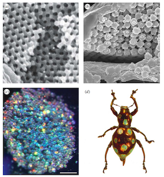
Last but not least, Dr. Ainsley Seago has surveyed the colorful nanostructured scales of hundreds of species in two lineages of beetles. Her results suggest that even though these surfaces exhibit many different optical properties, they’re all likely assembled as liquids in a process remarkably similar to the assembly of cell membranes (called lyotropic assembly).
The shiny, bright colors on beetles come from nanostructured scales. (Image courtesy of Dr. Ainsley Seago)
Image Analysis
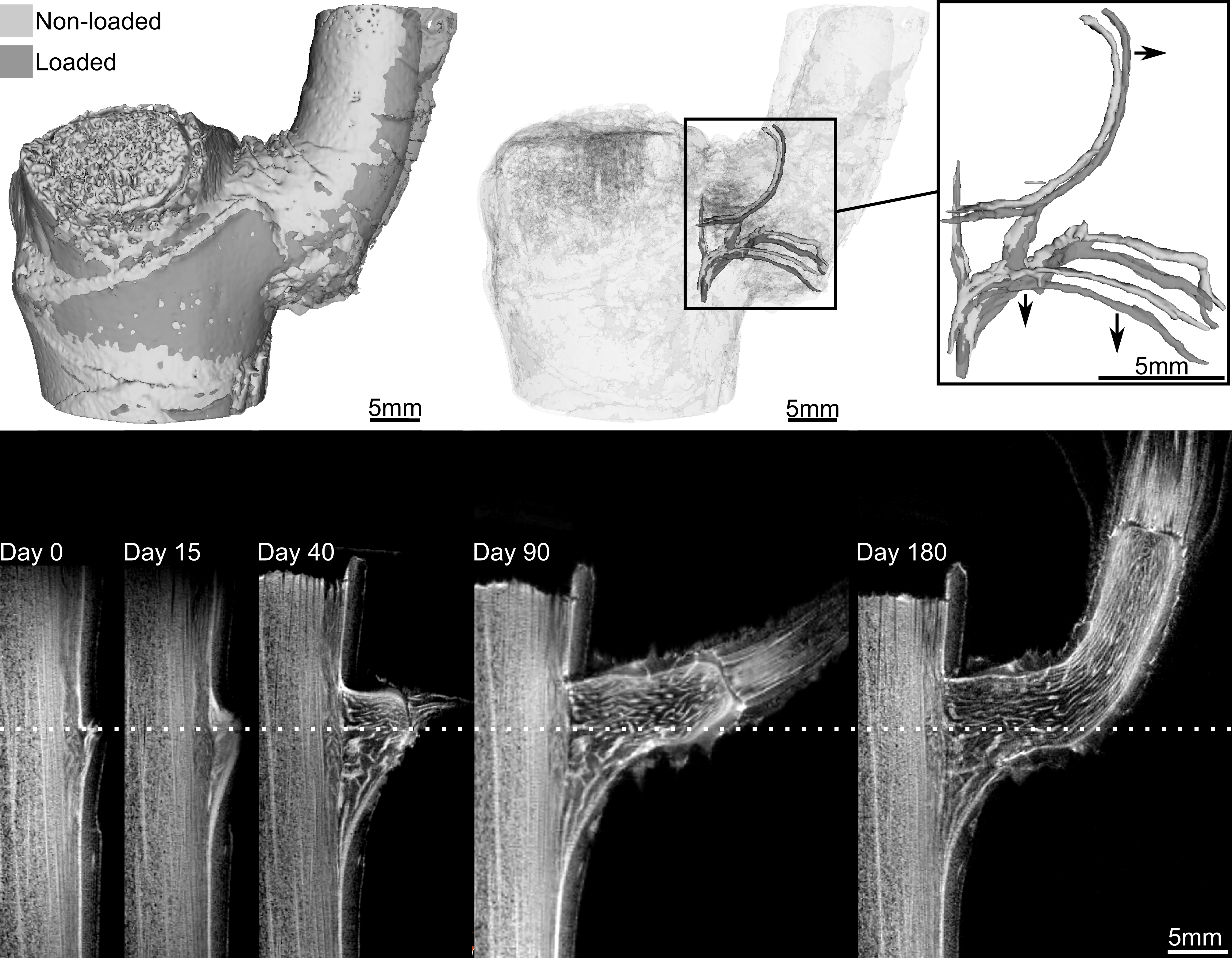
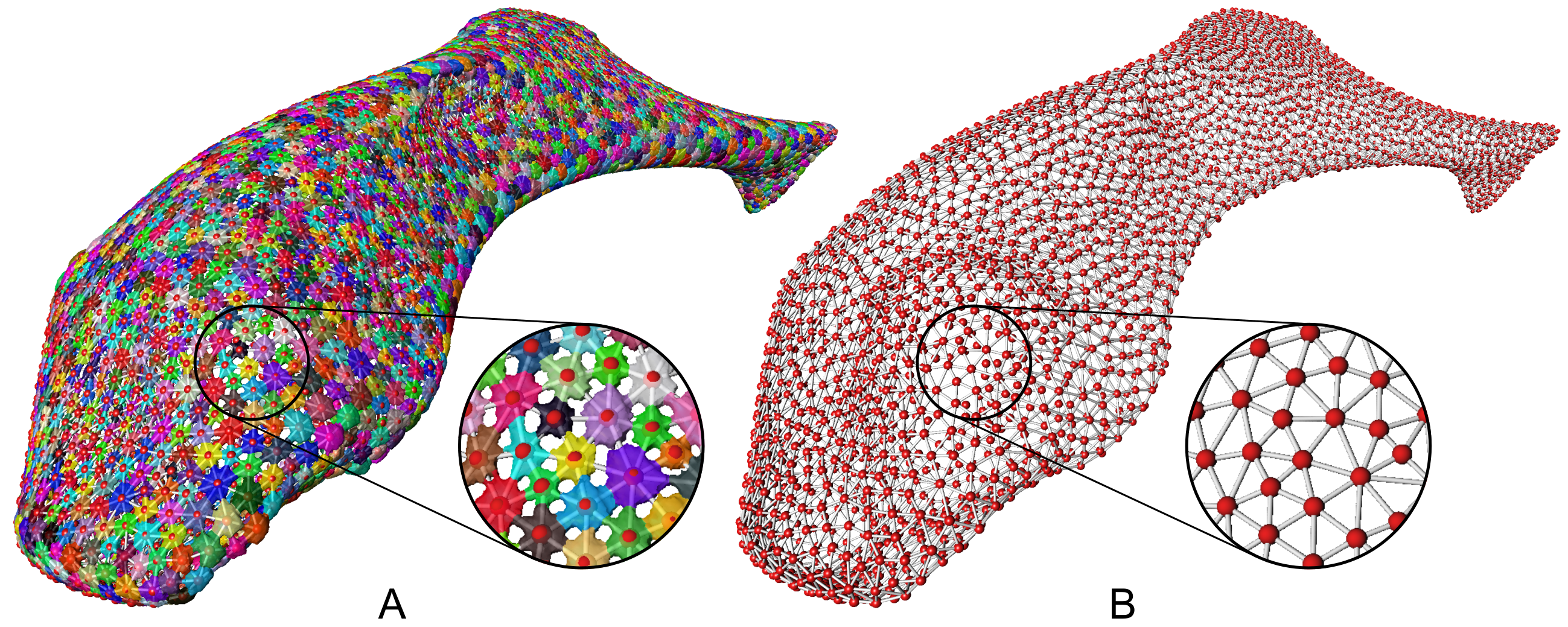
Dr. Daniel Baum is an expert on computational solutions for automated image analysis. He presented on common approaches for automatically selecting different parts of an image. This is really useful for studying material and biological systems with lots of similar repeating structures, and modeling how these systems respond to external forces. He presented examples of this work applied to the study of sharks and rays, whose soft cartilaginous skeletons are wrapped in a network of tiny, repeating, mineralized plates (called tesserae).
Computational methods, such as the watershed algorithm, can automatically segment different parts of an image and be used to construct 3D models of bones, cartilage, and other material. (Image courtesy of Dr. Daniel Baum)
Hierarchy
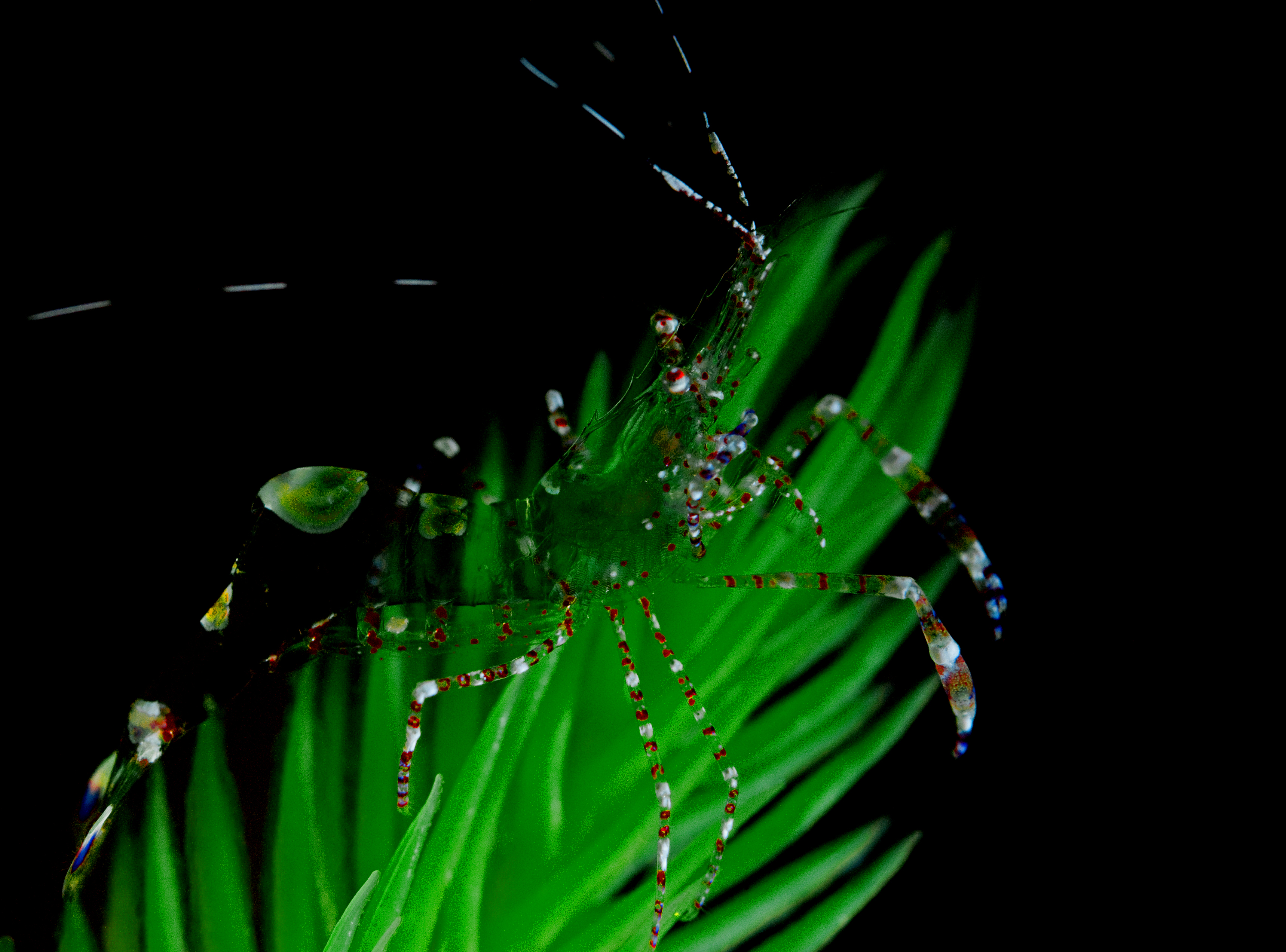
The layered organization of materials at different scales (forming a hierarchy of structure) is important for many biological materials’ properties. Dr. Laura Bagge studies invisibility in deep sea ocean life, and she presented how the size of the tiny microfibrils that make up larger muscle fibers can change how opaque an organism is — larger microfibrils have fewer interfaces for light to interact with, allowing the whole body of some shrimp species to be transparent.
These kinds of hierarchies are more commonly associated with strength, as in the example that Dr. Adam van Casteren presented. He studies how enamel, the outer layer of the tooth, resists wear, showing work suggesting that different levels of the material structure (nanostructure vs. microstructure) might respond differently to evolutionary pressure. That means that these hierarchies might have evolved to protect against damage from different types of diets, i.e. abrasion from sand particles in plant-based diets versus fracture from breaking apart bones and shellfish.
Transparent shrimp achieve invisibility by having larger muscle microfibrils. (Image courtesy of Dr. Laura Bagge)
Microfluidics
Fluid transport (both liquids and gases) is crucial for organism survival, so it’s no surprise that many biomaterials have been optimized for this function. Dr. Anna-Christin Joel presented work on how lizard scales and certain spider silks use capillary forces to manipulate fluids. The same capillary control has been harnessed to transport water droplets collected along the body to the mouth for drinking and to make capture silk stick more tightly to prey (by pulling waxes up from the surface of insects).
In a different application of fluid handling, Prof. Cassie Stoddard talked about the large eggs of emus. All eggs have pores that provide airflow to the growing chick, but the pores in emu eggs are forked not straight. This might help solve the challenge of getting enough breathable air into large eggs without weakening the shell enough that it could be crushed by the adult (interestingly this feature is also seen in dinosaur eggs!).
In my previous post on soft nanoparticles, you were introduced to polymer-based nanoparticles that could be used in biomedical applications, one of which is cancer therapy. These nanoparticles have a range of useful properties for cancer treatments, including their spherical shape and small size (~100 nm), both of which are similar to exosomes, small globules that are used in nature for transferring proteins between cells. Since cells naturally absorb exosomes, artificial particles with this size and shape should also be easy for cells to absorb, which means these particles could be used to deliver drugs into cells. While this idea sounds promising, it hasn’t worked out in practice — when drug-loaded polymer-based nanoparticles were injected into a tumor, subsequent tests showed that less than 1% of the injected dose entered the cancer cells. Since these particles were the correct size and shape, why didn’t they get inside the target cells?
One possibility is that the elasticity (or stiffness) of nanoparticles is to blame: scientists have suspected that this mechanical property can affect the ability of nanoparticles to squeeze themselves through the cell’s membrane. Unfortunately, it is difficult to test this hypothesis directly, because modifying the elastic properties of a nanoparticle generally requires modifying its chemical properties as well. To solve this problem, Peng Guo and coworkers designed a special kind of nano-objects — spherical nanolipogels — with tunable elasticity. In this paper, they proved for the first time that breast cancer cells take up soft, squishy particles more easily than they take up hard ones.
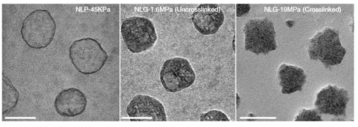
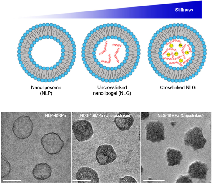
So what are nanolipogels? This type of nanoparticles is basically an altered version of a nanoliposome, a particle-like object that consists of a liquid water core surrounded by a layer of phospholipid molecules [1]. Guo and his colleagues created nanolipogels by filling the nanoliposomes’ liquid core with a polymer of tunable chemical structure. Nanolipogels have precise size (160 nm) and shape (spherical), and their elasticity can be made to vary without changing their other properties (see Figure 1).
Figure 1. Structures (top) and micrographs (bottom) of nanoliposomes and nanolipogels of increasing stiffness (higher values of Young’s modulus). (Image adapted from Guo’s paper.)
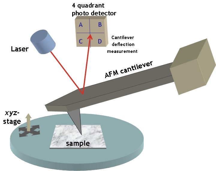
Figure 2. Experimental setup of an Atomic Force Microscope. The height of a sample’s surface is scanned by a tip on a moving cantilever and the cantilever deflections are detected by a laser light to give the samples topographic profile. (Image from simple.wikipedia.org)
To measure the elasticity of the particles they had produced, Guo and coworkers used a technique called Atomic Force Microscopy (AFM). AFM is commonly used to visualize soft materials by imaging the height of their surface through the deflection of a cantilever (Figure 2). In this paper, the researchers used AFM for a different purpose: to calculate the Young’s modulus — a measure of stiffness — of the nanoparticles. They did this by compressing the particles between the cantilever tip and a solid surface, allowing the researchers to measure the force required to deform the particles by some known amount. The relationship between the applied force, the degree of deformation, and the Young’s modulus is given by the Hertz equation [2]. What you need to remember is that the greater the modulus, the stiffer the particle.
The researchers created four different nanolipogels of different elasticity with Young’s moduli ranging from 1.6 MPa (roughly the stiffness of cork) to 19 MPa (the stiffness of leather), and a nanoliposome without polymer in the core with a Young’s modulus at 0.045 MPa (roughly the stiffness of gummy bears). After verifying that all 5 particles could successfully encapsulate drug molecules, they tested how well tumor cells could uptake each particle. To do so, they used breast cancer cells in the lab (in vitro cellular uptake) and attached fluorescent dye to the particles to determine whether they were inside or outside of the cells. They found that the stiffest nanolipogels were 80% less effective compared to the softest nanoliposome samples; in other words, five times more of the softer particles got inside the cells. In vivo tumor uptake studies, using live mice, similarly showed that the nanoliposomes had up to 2.6 times higher cellular uptake than the stiffest nanolipogels.
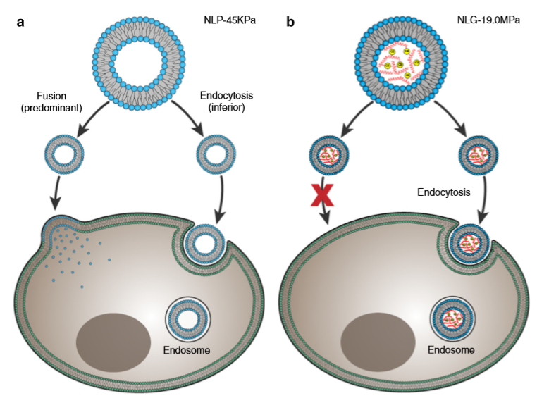
Why do the soft nanoliposomes enter the cells more easily? To understand the conclusion of Guo and colleagues, we need to think about how nano-objects enter a cell. Figure 3 shows two possible ways of doing this: 1. fusion, where nano-objects break up and join the cell membrane, or 2. endocytosis, where the whole object enters the cell by bending the cell’s membrane and getting covered in a membrane outer layer. Fusion needs less energy compared to endocytosis, where cell membrane bending and surface tension increase the energy. The researchers hypothesized that nanoliposomes use both fusion and endocytosis, with a preference for fusion (Figure 3a), while nanolipogels can only enter the cell through endocytosis (Figure 3b). This hypothesis was verified by using chemical compounds that prevented endocytosis from taking place; in all experiments, the cellular uptake of nanoliposomes was as high as before, while much fewer nanolipogels were detected in the cells, since they couldn’t enter through endocytosis.
Figure 3. The possible pathways of (a) nanoliposomes and (b) nanolipogels entering a cell. (Image adapted by the Guo paper.)
This study showed that a nanoparticle’s mechanical property, in particular, its elasticity, affects how it enters cells, a finding that could potentially have a tremendous impact on cancer treatment and diagnosis. The use of nanoliposomes, which are a synthetic equivalent of nature’s drug delivery systems, may also be used in the future to further understand how cellular processes, such as fusion and endocytosis, take place.
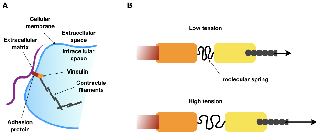
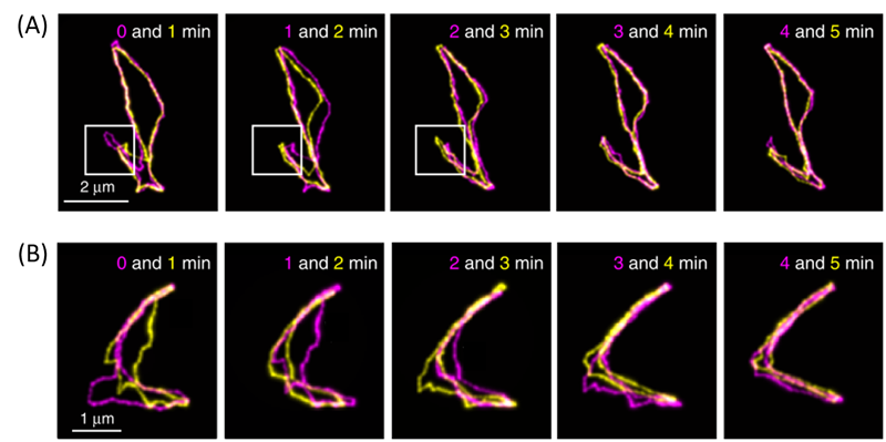
“USE YOUR LEGS!” That’s what might have been yelled at you the first time you went climbing. We are so used to walking or running that we don’t even think about how we do it. But when we face a new environment, such as a steep slope, we realize that finding the best strategy to move through space is not so easy. Now, imagine you are as small as few dozens of microns, without legs or arms, and you live in a viscous fluid. How would you move? This is the question biologists who are interested in cell movements have been trying to solve. By observing cells under a microscope, they saw that depending on their type or their environment, cells exhibit a wide variety of motion strategies. However, one thing never changes: cells need to exert forces on their environment to move. To do so, some kinds of cells create structures called focal adhesions. These structures are made up of several proteins, assembled on the outside of the cell. Like tiny bits of double-sided tape, their purpose is to stick the cell to whatever is nearby (see Figure 1). In slightly more technical language, focal adhesions connect the molecular skeleton of the cell to a substrate.
Figure 1. Movie of a moving cell with fluorescently labelled focal adhesions (from Berginski et al. 2011)
Cells can exert forces on their environment through focal adhesions. While it is possible to measure these forces outside the cell by engineering some force-sensing substrate [1], it is much trickier to understand what happens inside the cell. Accessing these forces inside the cells is the challenge Grasshoff and colleagues tackled in their 2010 paper.
In order to measure a force, the most straightforward method is to use a spring. A spring is a stretchable object for which, after calibration, we can relate its extension to the applied force. Therefore, a force can be measured by measuring the length of the spring. To measure the forces focal adhesions apply on the cell, one would need to inject tiny springs in the cells and connect them to the exerting-force structures.
To do this, the authors had the idea of taking advantage of a silk protein, produced by a spider, which is literally a molecular spring. Thanks to genetic tools, a part of the gene of this silk protein could be inserted within a gene called vinculin. The vinculin gene produces a protein that is an essential part of the focal adhesion structure. As shown in Figure 2A, vinculin connects the protein filaments of the cell skeleton to the outside of the cell (the extracellular matrix). The researchers engineered an artificial variant of vinculin that includes a molecular spring, derived from the silk protein, right in the middle of the naturally occurring vinculin molecule (see Figure 2B).
Figure 2.A. Schematic of focal adhesion. B. Schematic of the modified vinculin under low and high tension. Under high tension, the molecular spring is stretched. Red: adhesion protein, orange: vinculin head domain, yellow: vinculin tail domain, grey: contractile filaments. Arrows represent the magnitude of the tension.
After verifying that cells that are genetically modified to include the engineered focal adhesion protein behave normally, the next step was to measure the molecular spring extension. However, measuring distances at the molecular scale is not a piece of cake. For instance, the typical extension of such a spring is 6 nanometers, which is, by far, below the resolution of the best optical microscopes [2]. To circumvent this limitation, Grasshoff and colleagues took advantage of the Förster resonance energy transfer (FRET) effect to measure the distance between the two vinculin domains. The FRET effect takes place between two fluorescent molecules very close in space. A fluorescent molecule, when excited by a light at a precise wavelength, emits a light at a longer wavelength. But if a second fluorescent molecule is close enough, the first molecule (the donor) can directly transfer its energy to the second molecule (the acceptor). Then, the acceptor will emit light at an even larger wavelength than the donor’s. Consequently, the FRET intensity can be computed by measuring the relative emissions of the donor and acceptor molecules: the closer the acceptor is to the donor, the more energy the acceptor will absorb and re-emit. Furthermore, and importantly for this application, the efficiency of this process is very sensitive to the distance between the donor and the acceptor As a result, the distance between the two molecules can be measured with great precision (sub-nanometer) by measuring the intensity of the FRET effect. Therefore, the authors further engineered the vinculin protein by placing the molecular spring between two fluorescent molecules (Figure 3, yellow and red circles) that were capable of undergoing the FRET effect to measure the extension of the molecular spring.
Figure 3. Förster resonance energy transfer (FRET) effect in the modified vinculin of a focal adhesion under low and high tension. The excitation light of the donor molecule (yellow circle) is shown in green and the emission light of the acceptor molecule (red circle) is shown in red.
At this point, the authors had a method for measuring the tension intensity across vinculin molecules just by looking at the FRET intensity. In this way, they could generate a tension map across the contacts of the cell with its environment. They saw that focal adhesion under high tension leads to a growth of the size of the focal adhesion which relieves it from its high tension. Perhaps surprisingly, they also showed that regions where the contact is extending (protruding areas) are under higher tension than regions where the contact is receding (retracting areas), as shown in Figure 4.
In this paper, the authors developed a new technique to measure forces inside cells. By conducting single-molecule experiments, they even could calibrate their engineered molecular spring and relate the FRET intensity to absolute values of forces (in the order of a few piconewtons [3]), paving the way to a whole class of new FRET-based force sensors with different stiffnesses, which can now be used in other structures inside cells.
Everything started with adding a spider silk gene in a cell. Such mutant cells have the amazing power of shading light on the cellular force machinery. But “with great power, comes great responsibility” as another spider mutant has once been told.
Figure 4. The FRET index (ratio of donor to acceptor fluorescence) reveals the state of tension through vinculin across a cell. Close-ups retracting areas (R1 and R2) show a high FRET index, ie. a low tension, and protruding areas (P1 and P2) show a low FRET index, ie. a high tension (adapted from Grashoff et al.).
[1] These techniques are called traction force microscopy. The deformation of calibrated substrate (either a gel or micropillars) is measured to calculate the forces exerted by the cell. [2] Classical optical microscopes have a typical resolution of around 200 nm. New techniques of super-resolution microscopy reach a resolution of a few dozens of nanometers. [3] To give you a sense of this order of magnitude, when you hold a pen of, let’s say 10 g, you apply a force of 0.1 N. At the cellular level, cells exert on their environment forces in the order of dozens of nanonewtons (according to this study). At the molecular level, DNA has been manipulated applying forces in the same range as the vinculin tension: 1-100 pN (according to this study).


![Berginski M, Vitriol E, Hahn K, Gomez S [CC BY 2.5 (https://creativecommons.org/licenses/by/2.5)], via Wikimedia Commons](https://softbites.org/wp-content/uploads/2019/02/high-resolution-quantification-of-focal-adhesion-spatiotemporal-dynamics-in-living-cells-pone.0022025.s014.ogv.jpg)