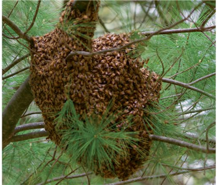
A honeybee colony can only exist when many individual bees cooperate. When a hive becomes too crowded, about 10,000 of the workers and a queen leave the hive to form their own colony. While the scout bees are searching for a new nest site, the rest of the bees are exposed to all of the dangers of the outside world, such as predators and storms, and have to stick together for protection. They form a “cluster”, which hangs on a nearby tree branch (as in Figure 1a) until a new suitable nest site is found. Sometimes, beekeepers hang these clusters from their faces as a “bee beard”.
In this study, Orit Peleg and colleagues investigated how these bee clusters stick together against the forces of gravity and the wind by shaking them and tracking how the shape of the cluster changed. Their experimental setup consisted of a board attached to a motor that shook it horizontally at frequencies between 0.5 and 5 Hz and accelerations up to 0.1 times gravitational acceleration. Peleg and colleagues put a queen bee in a cage attached to the board, leading the rest of colony to cluster around her, as shown in Figure 1b. Once the cluster formed, the researchers turned on the shaking and filmed how the bees behaved.
Figure 1. a) A bee cluster in the wild. The worker bees are protecting the queen until they find a new hive. b) A bee cluster in the lab, with the queen attached to the top board in a cage. Figure adapted from original article.
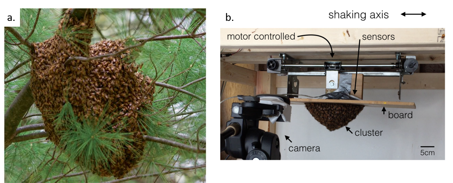
As the bee cluster was shaken horizontally, its tip swung from side to side at about 1 Hz, or one cycle per second. Peleg and colleagues tracked the bees moving from the tip of the cluster to the base as the cluster flattened over about 30 minutes. A flatter cluster does not swing nearly as much as an elongated one. Once the shaking was turned off, the cluster elongated again after 30 minutes to two hours, longer than it took the cluster to flatten. This is shown in Figure 2.
Figure 2. A honeybee cluster adapting to shaking filmed from the side and the bottom over time. While the shaking is on, the cluster spreads out along the base, and becomes shorter. When shaking is turned off, it returns to its original form. Figure adapted from original article.
Peleg and colleagues observed that individual bees responded to the variations in strain near them. At the base of the cluster, the strain was high, since the base bore the load of the entire swinging cluster. The bees at the base stretched their limbs to hold the rest of the cluster as it swung back and forth. The strain at the tip of the cluster was lower, since the bees there did not have to stretch as much to hold on. As more bees reached the base of the cluster, it flattened, making it swing less and decreasing the local strain on all the bees. The cluster was much flatter after 30 minutes of shaking, as in Figure 2. The bees at the base then didn’t have to stretch as much to hold on, and the cluster was safe from being torn apart. Even though an individual bee moved towards a greater strain, which may have been less comfortable for it, this collective bee behavior ultimately decreased the strain on the entire colony.
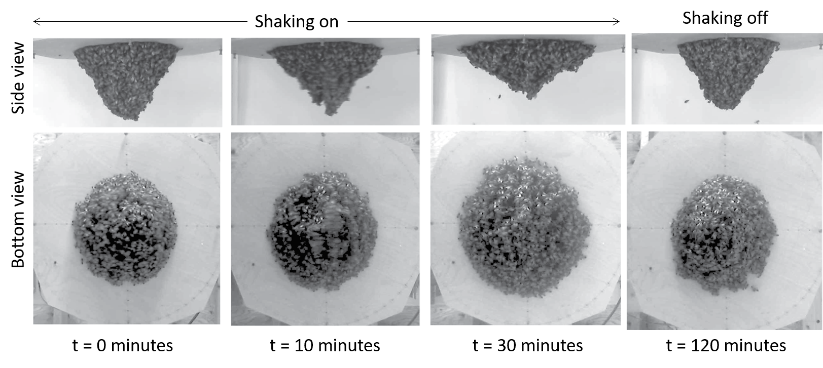
The researchers hypothesized that when a bee experienced a “critical strain”, a high value that might endanger the cluster, it moved to where the strain was higher — up towards the base —changing the cluster’s shape. To show that moving in the direction of increasing strain is a possible explanation for how the cluster flattens, Peleg and colleagues simulated honeybee clusters of different shapes under horizontal shaking (Figure 3). Each bee was modeled as a spherical particle experiencing gravity and attraction to neighboring bees. The simulated bees could not overlap with each other.
For their first simulation, the researchers simulated an entire cluster in 3D with stationary bees subject to horizontal shaking. They wanted to investigate the relationship between cluster shape and the strain. In this simulation, longer bee clusters experienced a higher strain when they were shaken, as shown by the color gradient in Figure 3a, with yellow corresponding to a higher strain than blue.
A second set of simulations allowed bees to break their connections with their neighbors and move in the direction of increasing strain if their neighboring strain was above a critical value. As expected, bees moved towards the base when shaking was simulated, and the cluster flattened out forming a shape similar to what was observed with real bees in Figure 2, shown in Figure 3b.
Figure 3. a) Three clusters simulated with horizontal shaking, from flat to elongated. Longer clusters have much stronger strains at the base. Blue colors correspond to lower strains while yellow corresponds to high strain. b) When shaking is turned on, simulated bees move towards higher strain (in the direction of the arrows) and flatten the cluster. Red and yellow colors correspond to higher strains. Figure adapted from original article.
This behavior lets bees keep the queen safe and the colony together on the tree when the cluster swings side-to-side in the wind. The cooperation of bees following simple rules lets the colony survive until it finds a new home.
For the most part of biology, it is form that follows function. Proteins are a perfect example of this — they are made of a sequence of amino acids (the protein building units), which are synthesized by the ribosome. Once synthesized, the long strings of amino acids fold up into a particular 3D shape or conformational state. Proteins take less than a thousandth of a second to attain their preferred conformational state (called “native state”) that — if nothing goes wrong — ends up being the same for a given sequence. This process is called protein folding. Explaining how a protein finds its folding preference out of all possible ways in such a short time is a longstanding problem in biology.
But, how do scientists know if – and when – a protein is in its folded state? The most straightforward way to do this is by observing its function — the way that a protein performs some biochemical task within the cell. If the protein is functionally active, then it has achieved its proper structure. However, most proteins are too small to observe directly without damaging the cell. To solve this problem researchers frequently use Green Fluorescent Protein (GFP), a protein that glows when it is hit by light of a specific wavelength. By attaching GFP to other proteins, researchers can see exactly where those proteins are at different timepoints. GFP’s stability, lack of interaction with other proteins, and non-toxicity make it an extremely popular candidate for visualizing protein localization. In other words, one “function” of GFP is to fluoresce. Today’s paper seeks to understand how structure correlates with function in GFP, one of biology’s most important tools.
To control the folding process, the authors used dual optical tweezers to mechanically stretch and relax the protein. Optical tweezers — as the name suggests — manipulate the position of particles (beads) using laser light. These beads are typically in the size range of micrometers. To apply forces on the GFP, the beads are attached to the protein via DNA “handles,” so that a DNA strand attached to the protein will stick to the DNA strand attached to the bead. These strands are then bound together ensuring that the force on the beads is transferred to the GFP. The construct looks as follows:
Bead – DNA – Protein – DNA – Bead
When the beads move apart, the protein is stretched to its maximal possible length (also called its contour length) and is unfolded, but when the beads get closer together, the protein folds back to its preferred structure. This process is illustrated in Figure 1.
Figure 1: The beads (circles) at each end are manipulated by laser beams and move back and forth. The DNA handles (purple) are attached to the GFP protein (green) that folds and unfolds turning to a functionally active and inactive state, respectively.
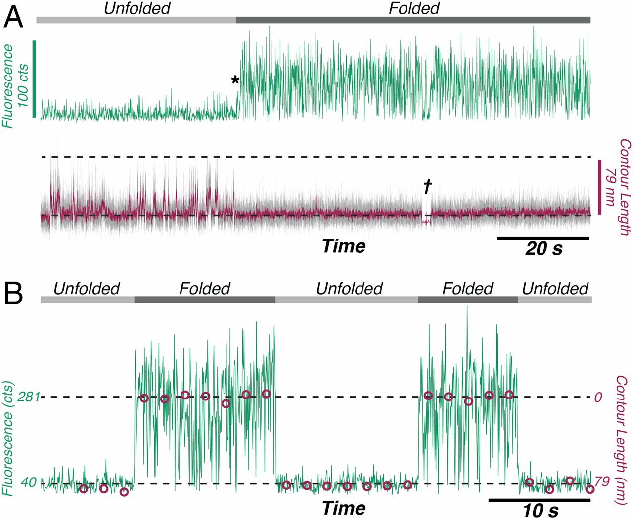
The authors observed that during unfolding, the GFP protein has undergone two intermediate states before unfolding completely. After unfolding, the beads were brought closer together and the protein folded itself back through the intermediate stages. The GFP molecule stopped emitting light when it was unfolded, which was expected. However, it started fluorescing only when it was completely in its folded state. This important finding showed that this protein is functionally inactive in any of the intermediate folding stages. The authors also observed that this process is reversible; they could unfold and refold the GFP molecule multiple times (see Figure 2).
Figure 2: Fluorescence signals of the GFP protein as it cycles through the unfolding and folding states. (A) The unfolded protein (light gray line) emits very little light (green signal) and its length fluctuates (purple line). Once the protein refolds (*) it emits more light and its length becomes shorter and consistent (dark gray line). † is the point where the force and state conformation are correlated(B) Cycled transition from dark (unfolded) to bright (folded). The purple circles represent the average contour length of each time. (Image adapted from Ganim’s and Rief’s paper).
These findings contribute towards understanding the functionality of proteins that could be used as in vivo optical sensors in force transduction. This work also opens up new avenues in studying biomolecules at the single-molecule level, such as DNA-protein complexes that can induce changes in conformation. Although the experiment only pulled the protein along one axis, this technique could be extended to pulling in several directions at once. If one could control the applied force in 3D, then it could be possible to gain more information on how exactly the protein folds and/or what happens during that process.
We are surrounded by phenomena caused by the scattering of light. When enjoying a sunny day at the seaside, like in the photo at the top, why is the sky blue? Blue light scatters more than red light. Why is milk opaque? Protein and fat particles scatter light. If you are reading this with blue eyes, your eye color is due to light scattering. Scientists use the same general scattering principle to study the structure of soft materials using the scattering of well-defined radiation. Scattering measurements reveal structures between an ångström and hundreds of nanometers, an important region for studying soft matter. Just as the color of the sky results from light scattered by air molecules, the scattering of X-rays and neutrons tells us about the size and shape of compounds in soft materials along with their interactions, and I will focus on these two types of radiation.
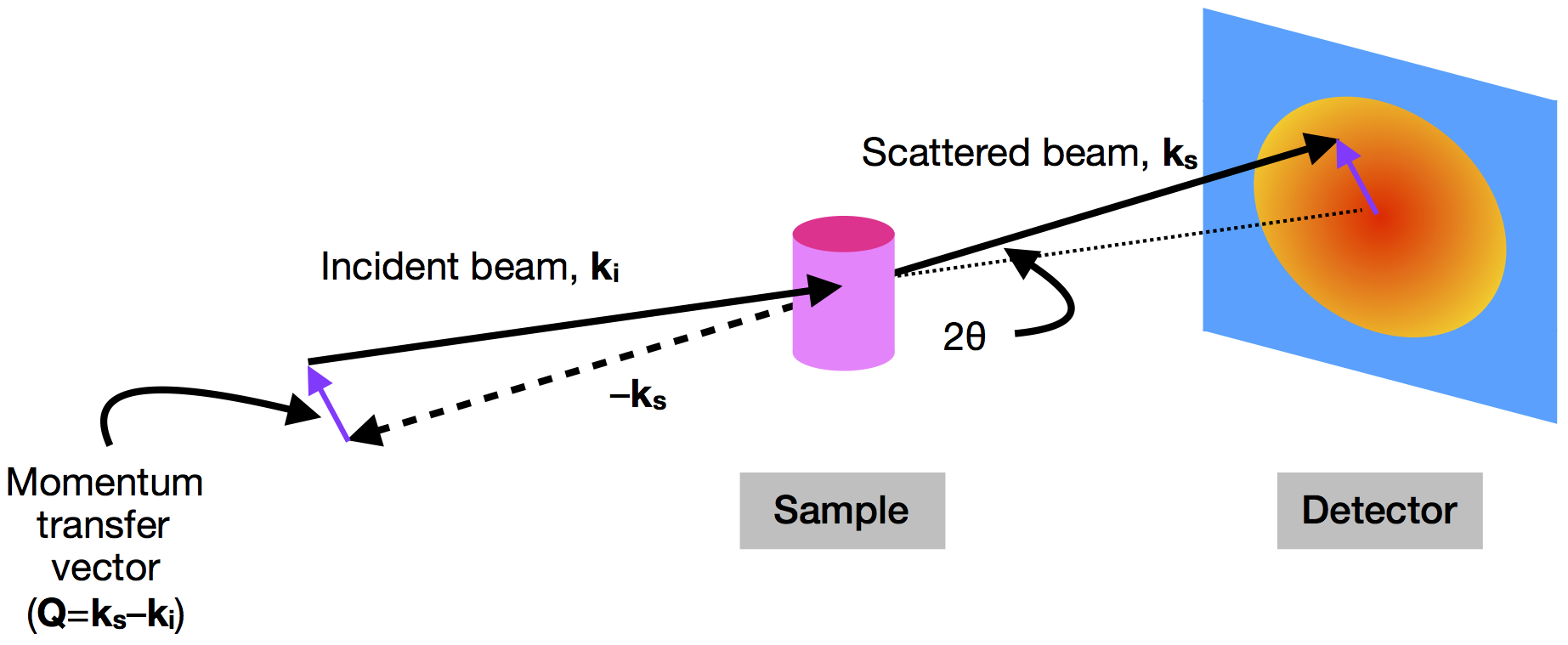
In a small-angle scattering experiment (SAXS when using X-rays and SANS when using neutrons), a sample (whether solution, dispersion, or solid) is placed between an incoming beam of radiation and a detector (see Figure 1) [1]. The detector measures the scattering intensity as a function of angle, which in turn can be related to the size and shape of the sample’s components.
Scattering intensity is quantified as a function of the momentum transfer vector (or scattering vector) $latex \mathbf{Q}$, which is simply the difference between the momentum of the incoming beam ($latex \mathbf{k_i}$) and the scattered beam ($latex \mathbf{k_s}$). The magnitude of $latex \mathbf{Q}$ (equal to $latex (4 \pi \sin{\theta}) / \lambda$) depends on the scattering angle ($latex 2 \theta$) and the wavelength of the radiation ($latex \lambda$) [2].
Figure 1. The geometry of a small-angle scattering instrument. An incident beam of X-rays or neutrons (with momentum $latex \mathbf{k_i}$) is scattered by a sample with an angle of $latex 2 \theta$. The scattered beam (with momentum $latex \mathbf{k_s}$) is then detected at a point beyond the sample. The difference in momentum between the incident and scattered beams is $latex \mathbf{Q}$. (Image produced by the author.)
The relationship between the magnitude of $latex \mathbf{Q}$ and the length scale being investigated ($latex d$) is given by the equation $latex Q = 2 \pi / d$, and this inverse relationship to distance is why measurements as a function of $latex Q$ are said to be in reciprocal space. (This relationship comes from Bragg’s law for crystals [3].) In real space, the arrangement of objects is described by the distances between them. In reciprocal space, the same arrangement would be given by $latex Q$. The scattering process is essentially a Fourier transform [4], a mathematical procedure to convert waves to frequencies, making it possible to go between real and reciprocal spaces.
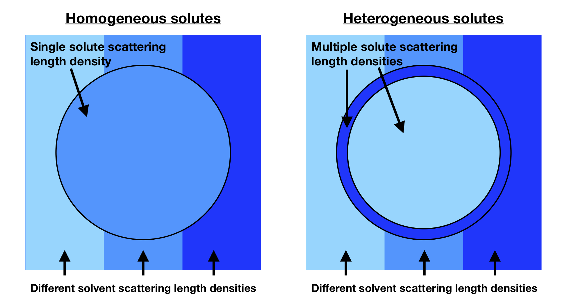
Now, having established some of the fundamentals of waves and scattering, we need to think about how radiation interacts with materials. This interaction determines the way that scattering data look and also what information you can obtain. Specifically, X-rays interact with electrons, and neutrons interact with nuclei. The magnitude of the interaction is quantified by the amount per volume (the “scattering length density”), and a difference in scattering length density between solutes and solvents results in detectable scattering. The scattering length density can be thought of as the “refractive index” for neutrons or X-rays. Figure 2 shows the general idea of contrast for any scattering experiment, with a comparison between homogeneous and heterogeneous solutes. When the color of the solvent and particle are the same shade of blue (meaning they have the same scattering length density), there is no scattering from that component. When the colors are different (meaning that they have different scattering length densities), there is now scattering.
Figure 2. Schematic of how the contrast between solutes (circle) and solvents (surrounding) for solvents and solutes with different scattering length densities gives rise to scattering. When the two colors are matched, which is possible for homogeneous solutes (left), there is no scattering. For heterogeneous solutes (right), there is no one solvent that can match the entire particle. (Image produced by the author.)
Interactions between X-rays and materials are fixed by their composition. However, neutrons interact differently with different isotopes of the same element. One particularly useful difference, especially for soft organic materials, is for structures with protons (1H) and those where protons are exchanged for deuterons (2H or D) [5]. It is possible to detect scattering from specific parts of complex systems by tuning the contrast of different components using solvents with different contrasts, as shown in Figure 2. Figure 3 shows calculated SANS (left) and SAXS (right) curves from chemically identical but isotopically distinct microemulsions, which are nanometer-sized droplets of water that are surrounded by surfactants in oil [6]. For the SANS curves, the dark grey areas represent deuterated oil or water (called D2O or heavy water), and the light grey areas represent standard hydrogenous oil or water. Multiple contrasts are required for a heterogenous particle, because no single solvent can match the whole particle (Figure 2, right). The curves are all different, but the actual structure of the microemulsion is always the same. It is only the contrast that differs. A precise determination of the structural dimensions of the microemulsion can be determined by analyzing all the data together, which gives more certainty than considering any one alone.
Figure 3. Scattering intensity as a function of the $latex Q$ for water-in-oil microemulsions calculated for SANS (left) and SAXS (right). For the three SANS curves measured, the dark grey regions are deuterated water (D2O) or deuterated oil, and the light grey regions are standard water (H2O) or oil. For drop contrast (red), you detect surfactant and water. For core contrast (blue), you detect water only. For shell contrast (green), you detect surfactant only. For the SAXS curve (purple), the contrast is fixed, and the water core dominates. (Image produced by the author.)
Scattering data is analyzed by comparing experimental data to known equations for how different shapes should scatter radiation as a function of $latex Q$. Luckily, many models are already known [7] for various shapes. However, as structures are determined somewhat indirectly from the scattering data, complementary information from other techniques, such as microscopy, is frequently obtained as well. The equation relating the shape and scattering as a function of $latex Q$ is called the “form factor”, an intraparticle property. For example, the curves in Figure 3 were all calculated using a form factor for a particle consisting of a spherical core surrounded by a shell of another material. At the extremes of $latex Q$, approximations can be used to calculate the size (at low-$latex Q$) and the interfacial roughness (at high-$latex Q$). In addition, the size distribution usually must be considered. In the example in Figure 3, the radii of the cores do not have a single value. There is a size distribution of about 20%.
For more concentrated dispersions or for more strongly interacting systems, the interactions between the particles must be considered. In these cases, an interparticle property called the “structure factor” contributes to the shape of the scattering curves. It can be calculated for particles that are considered to interact as hard spheres, charged spheres, or attractive spheres. Often samples are studied dilute to avoid the structure factor contribution. However, for systems that are necessarily concentrated or charged, it must be accounted for.
In this post, I focussed on the fundamentals of scattering with examples from nanoparticle dispersions in dilute conditions. However, these are not the only kind of soft materials that can be studied. Polymer solutions and blends, complex fluids, liquid crystals, gels, and a variety of biological materials (such as proteins and nucleic acids in solution or lipid bilayers) can be studied using small-angle scattering. The properties of soft materials often emerge out of their structures. By characterizing them in a quantitative way, scientists can determine the relationships between structures and their functions. Using small-angle scattering, we can not only better understand materials but also better predict ways of improving them. Small-angle scattering should be one of the tools employed by everyone interested in soft materials.
The featured image at the top is a photo of Bellevue Beach in Klampenborg in Copenhagen, Denmark. (Image taken by the author.)
[2] The angles being scattered are truly small, typically on order of 1° or less. By using $latex Q$, it is both the wavelength and angle that are important, and conveniently measurements performed using different wavelengths can be directly compared. ^
[3] Bragg’s law gives the conditions that a wave is diffracted by a series of planes. In a crystal diffraction measurement, peaks are observed in the data when Bragg’s law conditions are met. In a scattering measurement, where Bragg peaks are seldom observed, the relationship between $latex Q$ and $latex d$ is useful as a ruler for the length scale that is being examined. ^
[4] A Fourier transform is a mathematical operation that turns a periodic function, like a wave, into a probability of different frequencies. If, for example, you had a wave with a single wavelength, its Fourier transform would give a 100% probability at that wavelength. ^
[5] Deuterium is the heavy isotope of hydrogen with one neutron and one proton. ^
[6] A microemulsion is not just a small emulsion. Although, both are dispersions of two immiscible liquids, typically stabilized by a surfactant. A microemulsion is thermodynamically-stable and, in the case of a water-in-oil rather than oil-in-water, can be thought of as water-swollen surfactant micelle. Data for Aerosol OT-stabilized water-in-oil microemulsions can be found in the PhD thesis “Phase behaviour and interfacial properties of double-chain anionic surfactants” by Sandine Nave (University of Bristol). ^
Look inside a glass of milk. Still, smooth, and white. Now put a drop of that milk under a microscope. See? It’s not so smooth anymore. Fat globules and proteins dance around in random paths surrounded by water. Their dance—a type of movement called Brownian motion—is caused by collisions with water molecules that move around due to the thermal energy. This mixture of dancing particles in water is called a colloid.
Colloids are one of the classic topics in soft matter, a field of physics that covers a broad range of systems including polymers, emulsions, droplets, biomaterials, liquid crystals, gels, foams, and granular materials. And while I can keep adding items to this list, I can’t give you a precise definition for soft matter. I’ve never seen a completely satisfying definition, and I’m not going to even attempt to provide that here. But I can give you a taste of some of the definitions, and I hope you’ll come away with the feeling that you sort of know what soft matter is.
The phrase “soft matter” brings to mind pillows and marshmallows. These things fall under physicist Tom Lubensky’s definition (given in a 1997 paper) of soft materials as “materials that will not hurt your hand if you hit them.” And while many materials in soft matter are too squishy to hurt you, some of them might—cross-linked polymers can be pretty hard. And what about colloids? Slapping milk won’t hurt, but it also seems strange to call milk soft.
To understand what the “soft” refers to in “soft matter”, we first have to know where the name came from. The French term “matière molle” was coined in Orsay around 1970 by physicist Madeleine Veyssié, who worked in the research group of one of the founding fathers of soft matter, Pierre-Gilles de Gennes. The phrase apparently started as a private joke within the de Gennes group (don’t ask me what it meant), and the English translation of “soft matter” was popularized by de Gennes in a lecture he gave after winning the Nobel prize in 1991. De Gennes wrote that soft matter systems have “large response functions”, meaning that they undergo a large (don’t ask me how large) change in response to some outside force. So it seems we’re meant to take “soft” to mean something closer to “sensitive”, not necessarily soft in a tactile sense.
Now we can think about why colloids are soft from a different perspective. Remember that milk droplet under the microscope? The fats and proteins move around in the droplet due to thermal energy in the water; they are “sensitive” to the forces caused by thermal energy.
But even this “large response functions” idea doesn’t describe everything in soft matter. Some topics often considered a part of the field are concerned with general mathematical concepts instead of particular materials or systems. Take, for example, particle packing—the way particles arrange themselves to fit into confined spaces. Studying how particles can be arranged to pack on a curved surface is a mathematical problem and isn’t directly related to large response functions. However, since classic soft matter systems such as colloids are made up of particles you might want to pack, it makes sense to include packing as part of the field.
For every definition you give for soft matter, you can find a system that doesn’t quite fit. In an APS news article from 2015, Jesse Silverberg described soft matter as “…an amalgamation of methods and concepts” from “physics, chemistry, engineering, biology, materials, and mathematics departments. The problems that soft matter…examines are the interdisciplinary offspring that emerge from these otherwise distinct fields.” So maybe it’s not that important to have a rigid definition for soft matter; maybe its indefinability should be part of its definition. Soft matter is a field where the lines between traditional scientific disciplines are becoming ever more blurred—or, rather, soft.
In the world of engineering, crafting a material that meets the needs of your application is challenging. Often, a given material may only provide a handful of the required properties for that application. Instead, you may choose to combine two or more materials, forming a composite with all of your desired properties. In this week’s paper, Zhang and coworkers from the University of California at San Diego took a similar approach in the world of biology by combining a biomolecular crystal with a flexible polymer. The crystal provides structure to the composite and the polymer contributes to its flexibility and expandability. They showed that the composite could reversibly expand to nearly 570% of its original volume and unexpectedly found that it was self-healing.
Figure 1. A schematic of sodium chloride showing the repeating structure characteristic of an atomic crystal. Sodium and chloride ions are purple and green, respectively. [Image courtesy of Wikipedia]
Before we dive into the meat of this paper, let’s look at the properties of crystalline materials. An example is sodium chloride, also known as table salt, shown in Figure 1. You may immediately notice that the sodium (purple) and chloride (green) ions are precisely spaced apart from each other in a repeating pattern: a single sodium is surrounded by exactly six chlorides. This predictable structure is called a lattice. Many objects can form lattices if the interactions between neighboring objects can stabilize them. In the case of table salt, the crystal lattice is formed because sodium cations and chloride anions are oppositely charged, electrostatically attracting each other.
Figure 2. (A) The ferritin crystal structure. Each sphere is a single ferritin molecule. (B) A schematic of the close contact interactions between neighboring ferritin molecules, mediated by calcium (Ca2+). (C) A cutaway of a ferritin crystal demonstrating the porosity of the crystal. Images adapted from Zhang and coworkers’ original paper.
As mentioned earlier, biomolecules are also capable of forming crystals under right conditions. Ferritin is a hollow, spherical protein that is slightly negatively charged. As shown in Figure 2A, a given ferritin molecule is in direct contact with six other ferritin molecules, forming a lattice similar to table salt. You can see in Figure 2B that this lattice is held together by neighboring ferritins strongly interacting with calcium ions at the point where they come closest together. Because of the particular packing of the ferritin molecules caused by these interactions, a ferritin crystal is quite porous. Indicated by the arrow in Figure 2C, the pores between ferritin molecules are approximately 6 nanometers wide, large enough to allow water, salt solutions, and other liquids to soak into the ferritin crystal. In fact, the close contact interactions that stabilize the crystal are easily weakened when pure water is introduced into the pores, washing out calcium ions and dissolving the crystal. Instead, Zhang and coworkers wanted the crystal to expand but remain intact in water. Thus, they needed some kind of “glue.”
[wpvideo wlaJ8h1m]
Movie 1. A video of a hybrid crystal expanding when placed in pure water, followed by contraction after being placed in sodium chloride and calcium chloride solutions (by Zhang and coworkers).
They solved this problem by introducing a positively charged polymer into the pores of the crystal lattice. These polymers are known as hydrogels, as they can absorb a large amount of water and swell to many times their dry volume without dissolving away. Note that the hydrogel can’t prevent water from breaking the close contact interactions between the negatively charged ferritin molecules. Instead, the hydrogel holds the lattice in place to prevent it from dissolving due to electrostatic attraction between the hydrogel and each ferritin molecule. The close contact interactions can then be restored when a calcium salt solution is added. As shown in Movie 1, the authors demonstrated that the hybrid crystal could be expanded to nearly 570% its starting volume in the presence of pure water and returned to its original state when exposed to salt.
[wpvideo VfJcVEAF]
Movie 2. A video showing several examples of ferritin crystal cracking and healing upon expansion (by Zhang and coworkers).
Aside from the reversible expandability of this hybrid crystal, Zhang and coworkers unexpectedly found that it can self-heal. If the crystal expands too quickly, it tends to crack, as shown in Movie 2. Despite this, the authors noticed that the cracks often healed scarlessly over time. Hydrogels cannot typically self-heal on their own, unless explicitly designed to do so. In the case of the hybrid crystal, the hydrogel and ferritin molecules work in concert to heal cracks. The hydrogel does not allow ferritin molecules on each side of the crack to drift far away. Over time, these ferritin molecules then reform the reversible close contact interactions, thereby healing the crystal. However, this process seems to be somewhat imperfect, as the crystals tend to crack in the same spots upon repeated contraction and expansion.
In short, Zhang and coworkers were able to create a self-healing material with the structure of crystalline matter and the expandability typical of polymers. Further, these hybrid materials were unexpectedly self-healing after cracking during too-rapid expansion. Many crystals formed from proteins and other biomolecules are porous like ferritin and are stabilized by similar close contact interactions. These crystals could also be infiltrated with hydrogel and similarly made expandable and resilient. As Zhang and coworkers have done, rationally combining the properties of various classes of matter will allow the engineering of novel materials for a myriad of applications and with useful, and quite unexpected, properties.
You know how sometimes you tell to yourself things like “life is complicated”? Theoretical physicists are constantly reminded of this fact when studying living organisms. Recently, a new field of physics has emerged, inspired by the observation of living systems. What forces do cells exert during metastasis in cancer? What are the growth dynamics of biofilms of bacteria? How can a school of fish organize itself and move simultaneously? These are questions raised in the physics of active matter. Active matter is an assembly of objects able to move freely and capable of organizing into complex structures by consuming energy from their environment. Active matter can be composed of living or artificial self-propelled particles.
However, active systems differ from a simple gas or liquid because they are out-of-equilibrium. A system is in equilibrium if there is an energy balance between the system and the environment. When the energy isn’t balanced, the system will evolve toward an equilibrium state. Imagine a ball on a hilltop: it is in an out-of-equilibrium state until it has rolled down and stopped at bottom of the hillside. Now imagine that the ball is an active particle. This means it can consume energy from its environment to propel itself back up the hill, which drives the system out of equilibrium.
But physical notions such as pressure or temperature, are defined in thermodynamics only at equilibrium. This is why bridging the gap between physics and active matter has been a new challenge for theoretical physicists. Today’s paper focuses on the definition of a new quantity called swim pressure and highlights how researchers achieved its experimental measurements using an acoustic trap.
Rather than dealing with living organisms in this study, Sho and his collaborators used a system of artificial self-propelled particles, called Janus particles. They are made of two half faces; one in polystyrene and one in platinum [1]. Once immersed in a liquid, the platinum coating reacts with hydrogen peroxide contained in the liquid. The available energy resulting from this chemical reaction is then converted into motion. Particles move individually and randomly (analogous to an atom’s motion in a gas).
Due to self-propelled motion, active particles exert a mechanical force on their surrounding boundaries. In other words, a particle would naturally swim away in space unless confined by walls. The pressure exerted by active particles on the walls that confine them is theswim pressure. This is analogous to the definition of pressure from a microscopic point of view, which is the result of atoms colliding on a surface. Now that the theory is set, researchers try to measure swim pressure experimentally. But to control, confine and observe micro-particles between walls that you can remove at will is quite a challenge.
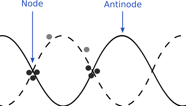
Figure 1. The curves represent two profile of an acoustic wave throughout time. Particles migrate to nodes due to the difference in acoustic pressure between nodes and antinodes.
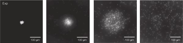
Sho and his collaborators at California Institute of Technology did not actually use physical walls in their experiment but instead used sound. When an acoustic wave propagates through a material, the deformation of the material causes a local pressure. Using this acoustic pressure, researchers can move objects between specific locations called nodes, which are special locations where the pressure wave is stable in time. The local pressure is minimal at nodes, while pressure is maximal at antinodes (see Figure 1). Since objects move from high to low pressure, the particles become trapped at nodes (see Figure 1). This technique is called an acoustic tweezer, or acoustic trap. Here, researchers built an acoustic trap such that many particles are confined over a large trap area.
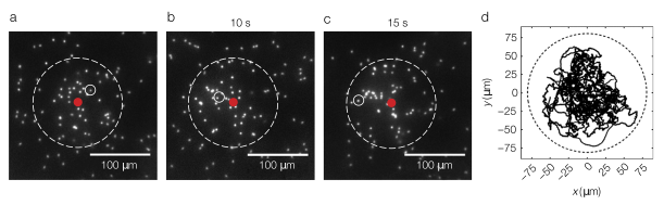
Figure 2: a-c. Snapshot of Janus particles in an acoustic trap (watch movie here). The red spot is the center of the trap and the white dashed line represents the contour of the acoustic trap. d. The figure shows trajectories of Janus particles moving randomly inside the trap (images adapted from Sho and coworkers’ original paper).
The researchers also adjust the size and force of the trap as a function of the velocity of active particles. Over time, more particles get trapped, and a densely packed cluster forms (see Figure 2). Particles can move within the trap area, but cannot exit (see Figure 2d). Then, when the acoustic tweezers are turned off, the cluster explodes! Meaning that free from confinement, active particles spontaneously disperse (see Figure 3). Thus, knowing the acoustic pressure and measuring the dispersion of particles over time allows researchers to measure the swim pressure.
Figure 3. Snapshots of Janus particles at different times after the acoustic trap has been released (watch movie here). The active cluster explodes, resulting in Janus particle dispersion (Images adapted from Sho and coworkers’ original paper).
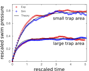
When you inflate a soccer ball with a pump, the walls will experience more collisions with the air molecules, meaning pressure increases. Similarly, squeezing the ball reduces space between the molecules and also results in an increase in pressure. These types of pressure changes are analogous to those observed in Sho and collaborators’ experiments. As shown in Figure 4, swim pressure increases over time as more particles get trapped (like pumping air into the soccer ball). Swim pressure also gets stronger for smaller trap area (like squeezing the soccer ball). But despite the analogy, we must not overlook the complexity behind the physics. Swim pressure is different from the pressure we experience every day, which comes from atoms and molecules. Here the classical model of pressure is an inspiration to build a new model. And as Figure 4 illustrates, the theory is consistent with experimental observations and validates this concept of swim pressure.
Figure 4. Evolution of the swim pressure as a function of time for two different size area. The swim pressure is higher for smaller trap areas. Researchers compare here experimental data with numerical simulations and theory (adapted from Sho and coworkers’ paper).
To conclude, today’s paper shows how classical physics quantities can be redefined to describe a new phenomenon in active matter. Sho and his collaborators used an ingenious device to measure the swim pressure exerted by active particles for different degrees of confinement and different crystal size. Their results confirm experimentally the theory of swim pressure established in a new approach of active matter, and open ways to a better description of the living world (from molecular to cells dynamics, bio-films formation, collective motion…). So indeed, life might be complicated, but from the point of view of scientists, this is what keeps them excited.
[1] these particles were named Janus particles in reference to the Hall-faced Roman God Janus.
We’ve all been there. We try pouring ketchup onto our fries from the bottle, but it doesn’t come out. So we tap the back of the bottle a few times, and suddenly, the ketchup rushes out and your entire meal is covered with it. Why does the ketchup exhibit such behavior?
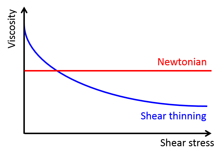
This behavior is called shear thinning, and only some special fluids exhibit it. For fluids, such as water and alcohol (these are called “classical” or “Newtonian” fluids) viscosity only depends on temperature. Therefore, if the temperature doesn’t change, the viscosity remains constant (see the red curve in Figure 1). However, in non-Newtonian fluids, viscosity depends on another variable called the shear stress. Shear stress is the stress felt by materials when they undergo deformation caused by slip or slide. In shear-thinning fluids, which are a type of non-Newtonian fluids, the viscosity decreases when the shear stress increases (see the blue curve in Figure 1). Ketchup, with other suspension fluids such as blood and nail polish, falls into this category of shear-thinning fluids. So, by tapping the ketchup bottle, we apply shear stress to the ketchup inside, causing the viscosity to drop and making the ketchup flow out of the bottle. But, even though this phenomenon has been on scientists’ radar for a long time, the microscopic mechanism for shear thinning is still unknown for certain fluids.
Figure 1. Shear stress vs. viscosity of Newtonian and shear-thinning fluids.
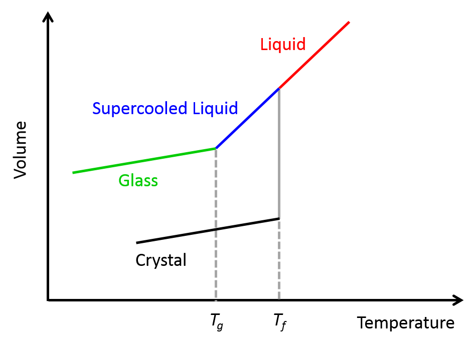
Another type of fluid that exhibits shear-thinning behavior is the “supercooled” liquids. As shown in Figure 2, when a liquid – any liquid – is rapidly cooled below its freezing point, instead of crystallizing and solidifying (like what we typically see when water freezes in an ice-cube tray), it forms a supercooled liquid. When the temperature of this highly viscous liquids drops even further below its glass-forming temperature, it turns into a disordered glass-like phase [1]. That is why supercooled liquids are also called glass-forming liquids.
Figure 2. The relationship between the volume of liquid and supercooled liquid. Tf and Tg indicate freezing point and glass-forming temperature, respectively.
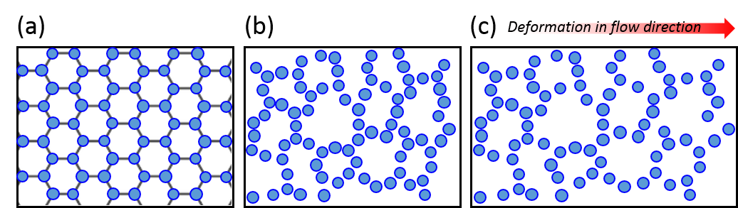
To understand the flow behavior of supercooled liquids, Trond Ingebrigtsen and Hajime Tanaka of the Institute of Industrial Science at the University of Tokyo ran molecular dynamics simulations. Molecular dynamics simulation is a computational method for studying the interactions of atoms or molecules. From the simulations, Ingebrigtsen and Tanaka were able to confirm what other scientists had previously suspected: shear thinning is linked to the increase in structural disorder of the liquid molecules (as illustrated in Figure 3(a) and 3(b)). To be more specific, it is linked to the structural disorder of molecules in the flow direction.
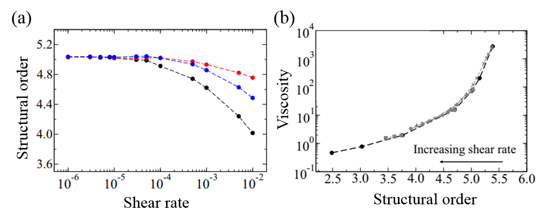
As a model for supercooled liquids, the authors chose to simulate a colloidal system, where molecules interact in a similar way to realistic fluids. After verifying that the simulates system acts like a supercooled liquid (for example, its viscosity decreases with increasing shear rate), they investigated the origin of shear thinning using this model. The molecular simulation revealed that as the shear rate increases, the molecular structure becomes more disordered. This is illustrated in Figure 3(a) and 3(b). More notably, the structural disorder was more prominent in the direction of the fluid flow compared to the structural disorder measured in any other directions relative to the flow. This can be seen from the black line of Figure 4(a), where the steep decrease of structural order could be observed with increasing shear rate.
Indeed, the structural disorder turned out to be the culprit behind the shear-thinning behavior in supercooled liquids. As shown in Figure 4(b), when the molecular structure becomes more disordered, the viscosity of the liquid decreases, a behavior expected in shear-thinning fluids. To understand this result, let’s picture molecules in the fluid. The shear applied in the direction of the flow would open up more space for molecules to rearrange themselves as the fluid expands, like it is shown in Figure 3(c). This leads to the decreased viscosity and the easier fluid flow.
Figure 3. (a) Structurally ordered molecular system. (b) A molecular system with increased disorder. (c) System after shear deformation in the flow direction.
Figure 4. (a) Shear rate versus structural order of the supercooled liquid model used in the molecular simulation. The black line represents the flow direction (blue and red each represents other two directions relative to the flow.) (b) Structural order versus viscosity. (Note the log scale on the y-axis.) All figures are adapted from the original paper.
This study sheds light on the previously unknown mechanism of shear thinning in supercooled liquids. Ingebrigtsen and Tanaka, however, insert that the microscopic mechanism for their observation should be further studied to fully understand the shear-thinning behavior. So, next time a disaster happens on your fries, chill out and think that you are just carrying out a super cool non-newtonian experiment!
(This post was updated on March 4th, 2020 to answer a comment that was made on the French translation of this post.)
[1] Technically, glass isn’t a phase, though I used that word for simplicity. Glass is an amorphous solid that has a disordered molecular structure (unlike ice, which has a well-defined crystalline structure). See Figure 3(b) for a visualization of a disordered molecular structure.
The shape of a container can affect the flow of the fluid inside it. Water in a narrow stream flows smoothly, but once the water molecules make their way into a pond, they spread out and no longer flow coherently. If you blow into a long, narrow straw, the air will go straight through. Once the air flows into the large room you are standing in, it slows down as it mixes with the air around it, so someone standing five feet away from you won’t feel a breeze at all.
The above examples show how the shape of a container affects the flow of passive fluids. In today’s study, Kun-Ta Wu and colleagues investigated how the motion of active fluids, fluids that flow using an internal source of energy, is also affected by the shape of their container. They used a system of microtubules, chains of proteins assembled into long, stiff rods. Clusters of a protein called kinesin exert a force on microtubules by “walking” along them. Microtubules interact with each other to form swarms or turbulent-like flows.
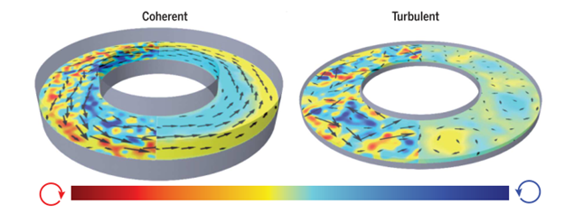
Wu and colleagues created 3D toroidal racetracks with rectangular cross-sections to confine the microtubule bundles. They saw coherent flows in racetracks with square cross-sections, but if the channels got either too thin and wide or too tall and narrow, the flow became turbulent (Figure 1). This result is described in this Softbites post from last year.
Figure 1: Comparison of coherent and turbulent flows around a track. The left side of each track shows the motion in an instant, while the right side shows the average motion over a long time. The color represents the local direction of spinning and the black arrows indicate the direction of motion. Microtubules in a red spot are spinning clockwise, those in a yellow spot are not spinning, and those in a blue spot are spinning counterclockwise. Image adapted from original article.
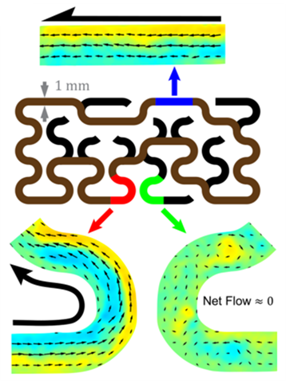
After Wu and colleagues got microtubules to flow by themselves, they placed them in increasingly complicated tracks. Active flows happened in any closed loop with an approximately square cross-section. Microtubule flows solved a maze, as in Figure 2, by flowing through the connected straight and curved sections, but not sections leading to dead ends. The dead ends slowed down the flow in the connected sections to about half the speed of a toroidal racetrack with an equivalent length.
Figure 2: Microtubules flow in straight and curved sections of the maze in closed loop, and no net flow loop in sections leading to dead ends. Black arrows show the direction of the flow and colorful arrows point to sections at which mean flows are measured. Figure adapted from original article.
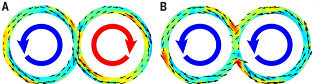
Wu and colleagues then created tracks made out of overlapping tori, or donuts. In the tori, microtubules spontaneously flowed in the same or in different directions, as in Figure 3. When the active flow was clockwise in one torus and counterclockwise in the other, the direction of flow in the overlap was the same, and the flow kept going (A). When they were both counterclockwise, two flows came into the overlap in opposite directions, and there was no flow in between the tori (B). Watch a video of this here.
Figure 3: Microtubules can flow in connected tori in (A) the same direction and (B) opposite directions. Figure adapted from original article.
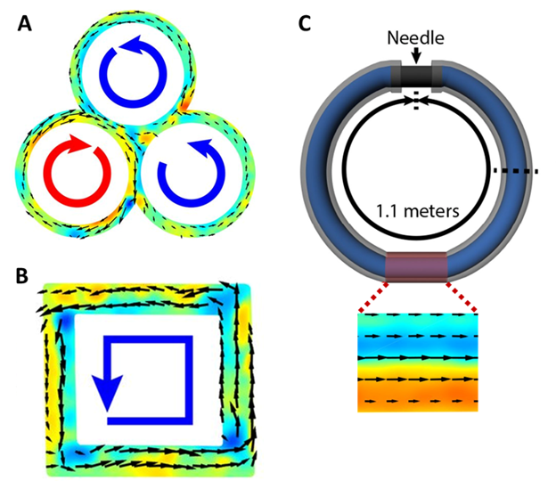
Microtubules created an active flow when a third torus was added (Figure 4A). They also navigated a square racetrack, although the corners created small vortices and slowed them down (Figure 4B). Finally, microtubules still flowed in a very long torus made out of a 1.1 meter-long tube joined at the ends by a needle (Figure 3C).
Figure 4: (A) Flows in 3 overlapping tori. (B) Microtubules flow around a square racetrack in the direction of the blue arrow. (C) Microtubules even flowed around a very long (1.1 meter) track. The closeup shows a time-averaged flow inside a small section of the tube. Figure adapted from original article.
Thus, these flows of microtubules aren’t just a one-time phenomenon that’s hard to replicate—no matter how much the researchers changed the system, as long as there was a closed loop with an appropriate cross-sectional aspect ratio, there was a flow.
These flows inside channels are interesting—but are they useful? The researchers suggest that a system like this could act as an internal power source for very small devices, but this application is still far in the future. It is also possible that a similar motion is used inside living cells to transport materials in a process called cytoplasmic streaming. More importantly, these flows are a beautiful example of collective motion induced by physical forces, helping scientists elucidate how swarms can form at all length scales.
Softbites team introduces its official authors. Find here our second post of our series of interviews. You can read Danny’s posts here.
Who are you and what is your research focus?
I am a physics Ph.D. student at Yale University studying theoretical biophysics. I use biology to inspire my search for new ideas in physics and use that new physics to learn new biology. Specifically, I study entropy production in an attempt to understand how biological systems use and dissipate energy.
Can you describe this picture illustrating your research?
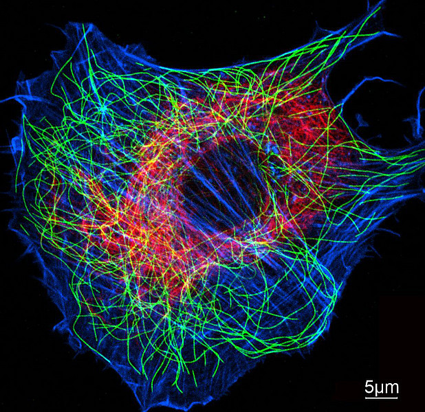
I primarily study the cell cytoskeleton, so it is fitting for the image to be from the cover of a recent textbook edited by Thomas D. Pollard (Yale) and Robert D. Goldman (Northwestern) called The Cytoskeleton. The image itself was provided courtesy of Harald Herrmann (University of Heidelberg). It shows a microscopy image of a cell with different components of the cytoskeleton labeled with fluorescent proteins — actin (blue), microtubules (green), and intermediate filaments (red).
Microscopy image of a cell with different components of the cytoskeleton labeled with fluorescent proteins — actin (blue), microtubules (green), and intermediate filaments (red).
Why do you think the science you do is important?
The work I do is very basic research — it doesn’t have an immediate practical impact that I can think of. However, uncovering exactly how cells use energy is an important step not only towards understanding biology, but can also lead to design principles to be used in micron-sized, soft, engineered materials. Also, from a pure physics point of view, we don’t understand out-of-equilibrium systems anywhere near as well as we understand equilibrated systems, and living things are about as far from equilibrium as you can get.
When did you first know you wanted to be a scientist and what were the crucial steps that took you to your current project?
I didn’t know I wanted to be a scientist until halfway through my first year of college. I entered school wanting to study music and business, but a class in acoustics quickly converted me to pure physics. I didn’t know what research was until my fourth year, but once I got a taste I knew I wanted to do more. I started out doing experiments in a soft matter lab studying colloids (micron-sized plastic spheres in water) under the mentorship of another Softbites writer, Christine Middleton (Hi Christine!). I found cells to be more interesting versions of colloids and decided to study biophysics in graduate school.
I was turned on to my current project for both practical and esoteric reasons. My moonshot idea of what I want to do with science is to identify a transition in matter from living to non-living in the same way we understand the transition from water to ice. This highfalutin idea has led me to the realm of understanding cells as information processing units, which requires understanding how they dissipate energy to process information. It turns out that a project in my lab had a very natural extension towards understanding energy dissipation, and I was able to put my interests to practical work in understanding biological experiments.
Danny Seara, Ph.D. student at Yale University
What are you passionate about outside of science?
My most recent obsession has been the impending water crisis that many cities around the world will soon face (the Vox Netflix show “Explained” has an episode about this that I highly recommend if you want to scare your pants off). I’m also interested in the intersection between science and law (this might be cheating out of the question), and in particular have begun researching how the idea of “universal laws” play a role in science, law, and in the dialogue that the two try to have on the issues mentioned above. I also play guitar and love hip-hop music.
Why did you choose to write for Softbites?
I did my undergraduate degree in the history and philosophy of science, so I spent a lot of my time writing. In grad school, there’s less opportunity for non-scientific writing and I wanted to exercise those muscles again. I care a lot about science communication and believe in the mission of Softbites to educate people on the ubiquitous yet often overlooked science of soft matter (which encompasses biological matter). It’s a fascinating subject I want to help popularize, and I like doing the work that goes into that popularization.
Softbites team introduces its official authors. Find here the first post of our series of interviews. You can read Olga’s posts here.
Who are you and what is your research focus?
I’m a Ph.D. candidate in mechanical engineering at Georgia Tech studying the biomechanics of maggots – specifically, black soldier fly larvae. These larvae eat twice their body weight per day in food waste. They are raised by startups all over the world as a source of sustainable chicken and fish feed. I study how these larvae eat so much, the physics of their interactions with each other and their environment, and how to better raise them in industry.
Here is an up-close picture of a black soldier fly larva.
Why do you think the science you do is important?
This research is important for two reasons. First, it will help find methods for startups to raise larvae better, so that they can be a sustainable and economically feasible source of protein. Second, this project is an example of “active matter” — how groups of self-propelled particles interact with each other and move in interesting ways. The collective motion of fly larvae, bacteria, and birds in flocks have a lot in common, and I am investigating the physics that leads to that.
When did you first know you wanted to be a scientist and what were the crucial steps that took you to your current project?
I’ve been interested in science all my life. I went to college for engineering but quickly realized that I love discovering how the world works even more than designing new technology. When I realized I could use my engineering skills to understand how animals move, I knew I was on the right track.
Olga Shishkov, Ph.D. student at Georgia Tech
What are you passionate about outside of science?
When I started my Ph.D., I also started doing aerial silks. This hobby is both great exercise and a fun distraction. I can’t worry about a paper or exam while hanging on to a piece of fabric by one hand upside down 15 feet in the air!
Why did you choose to write for Softbites?
I have really bad science FOMO. Whenever I read about an exciting new study, I wish I was working on what I just read about. However, I can’t just abandon the work I’m doing on my maggots! Writing about the papers I enjoy reading lets me explore them enough to get back to my work. I also really enjoy writing, and as a Softbites writer, I can write with a more fun style than in an academic paper. Finally, it’s important to communicate science to the public, and soft matter needs more attention from the science communication community.