Original paper: Stopping transformed cancer cell growth by rigidity sensing
Our bodies are made up of cells that can sense and respond to their dynamic environment. As an example, pancreatic beta cells chemically sense increased blood sugar concentrations and respond by producing insulin. Scientists have found that cells can also mechanically sense their environment; “mechanosensing” determines whether a cell should grow or die. Cancer is characterized by uncontrolled cellular growth, where cells often contain mutations that inhibit the natural mechanisms of cell death. Because mechanosensing is one such mechanism, scientists have hypothesized that cancer cells keep growing because they lack the ability to probe their environments. In this week’s paper, published in Nature Materials, an international research team led by Bo Yang and Michael Sheetz from the National University of Singapore investigated that hypothesis by combining tools from soft matter physics and biology.
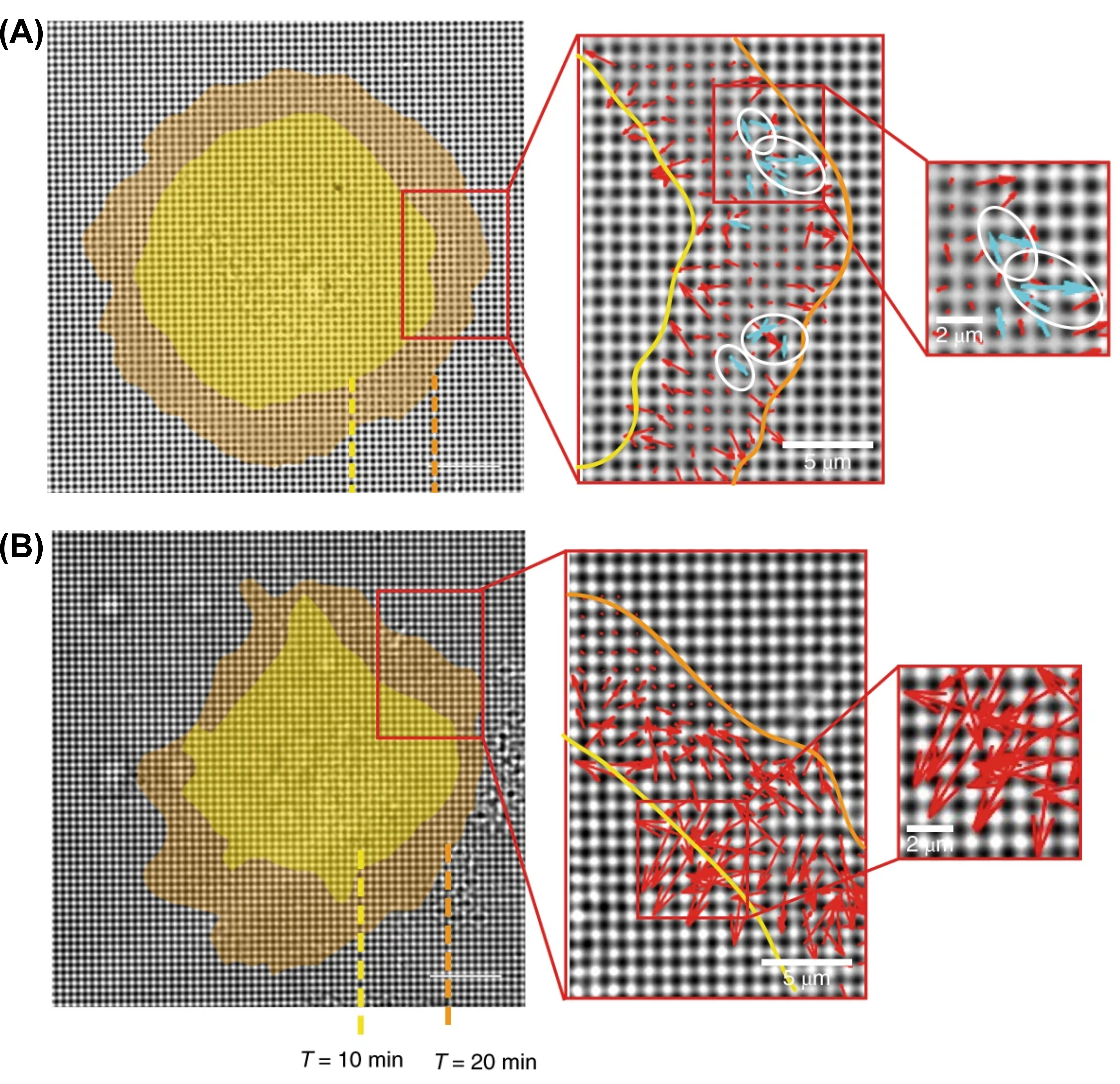
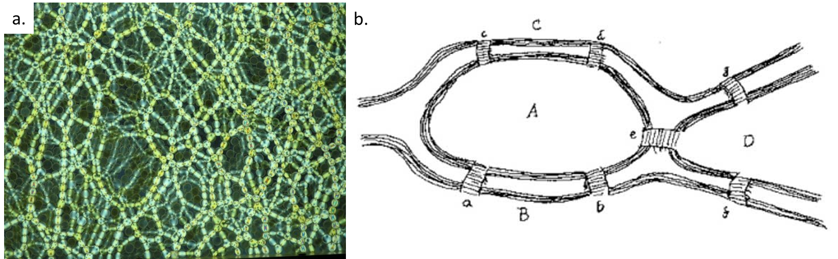
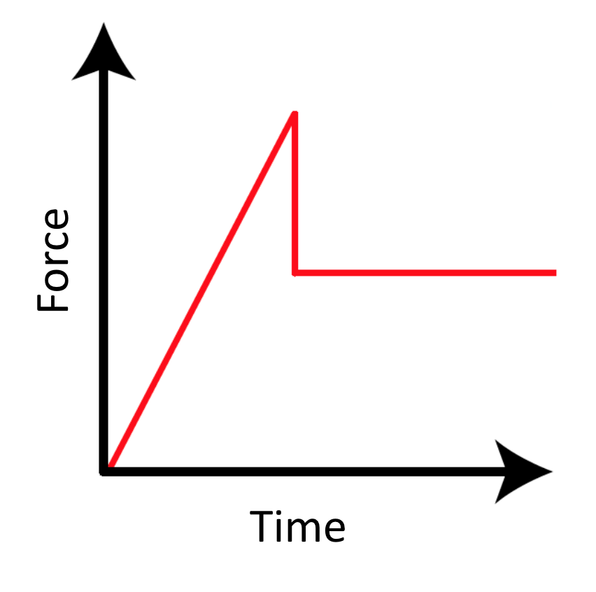
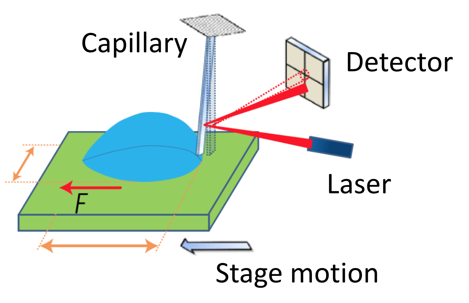
The team of researchers measured how well normal and cancer cell lines were able to mechanically probe their environments. To test cellular mechanosensing, they placed cells on a substrate consisting of microscopic pillars (500 nm diameter) made of polydimethylsiloxane (PDMS), a common polymer used in contact lenses. The pillars were coated in fibronectin, a protein that acts like a glue to help the cells stick to the pillars. From prior work, the researchers anticipated that cells would probe the rigidity of the PDMS pillars by pulling pairs of them towards each other. By measuring how much the cells bent the pillars towards each other, the scientists determined the forces exerted by the cells. As shown by the red arrows in Figure 1, both cancer and normal cell types deformed the pillars. However, only normal cells probed the rigidity of the substrate by pulling pillars together (blue arrows in Figure 1A). To evaluate the universality of their findings, researchers studied a variety of tissues derived from humans, monkeys, and mice. They found that normal cells from multiple species and tissues produced significantly more paired pillars than cancer cells, which confirmed that normal cells are universally better at mechanically sensing their environments.
Next, the researchers correlated their findings with the ability of cells to tailor their growth patterns depending on the rigidity of their environment. They found that normal cells died when placed on soft surfaces, such as soft agar, but grew when seeded on more rigid ones. Contrarily, cancer cells divided, and eventually formed colonies no matter how soft the surface was. From these results, it was proven that the loss of mechanosensing ability is highly related to the uncontrolled growth of cancer cells.
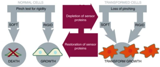
To confirm this finding, Yang and coworkers restored mechanosensing in cancer cells, expecting that doing so would also restore normal growth patterns. Normal cellular mechanical sensing is performed by protein complexes that can tug and pull on the cells’ external environment. The researchers noticed that cancer cells lacked proteins vital to the formation of these complexes. As outlined in Figure 2, when the activity of these proteins was restored, the cancer cells resumed growth patterns that were similar to normal cells. The researchers were able to subsequently cancel out the activity of other proteins, thereby reintroducing abnormal, cancer-like growth. By depleting and restoring proteins, researchers could turn cancer-like growth on and off reversibly and demonstrated that those proteins are vital in ensuring normal cellular growth.
In short, Yang and coworkers showed that normal and cancer cells differ in their ability to mechanically test their environments. Unlike normal cells, cancer cells were unable to differentiate between soft and rigid surfaces and kept growing in an uncontrolled fashion. However, upon restoring key sensing proteins, cancer cells grew and died similarly to normal ones. These findings may affect future cancer treatments; by restoring the ability of cancer cells to mechanically sense their environment using genetic tools, we may have one more method to limit or stop uncontrollable cell growth. Such a treatment would be invaluable in saving the lives of many.