Trichoplax adhaerens: tropical sea-dweller, microscopic contortionist, and biomechanical marvel

Original paper: Motility-induced fracture reveals a ductile-to-brittle crossover in a simple animal’s epithelia

Content review: Heather Hamilton
Style review: Pierre Lehéricey


Figure 1: The dynamic range of T. adhaerens with size ranging from 100 microns to 10 millimeters. Snapshots taken from live imaging. Images courtesy of the original article.

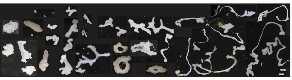
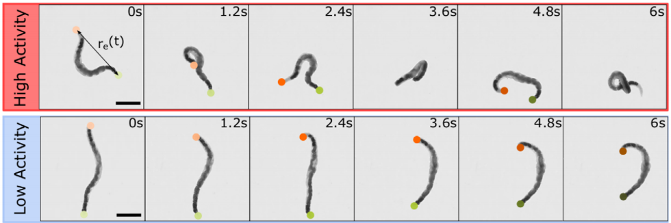
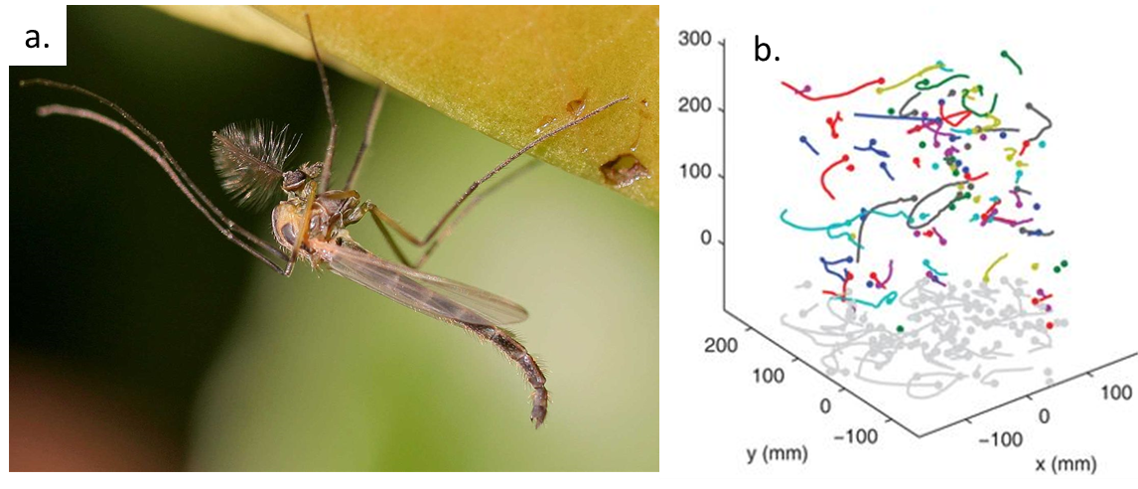
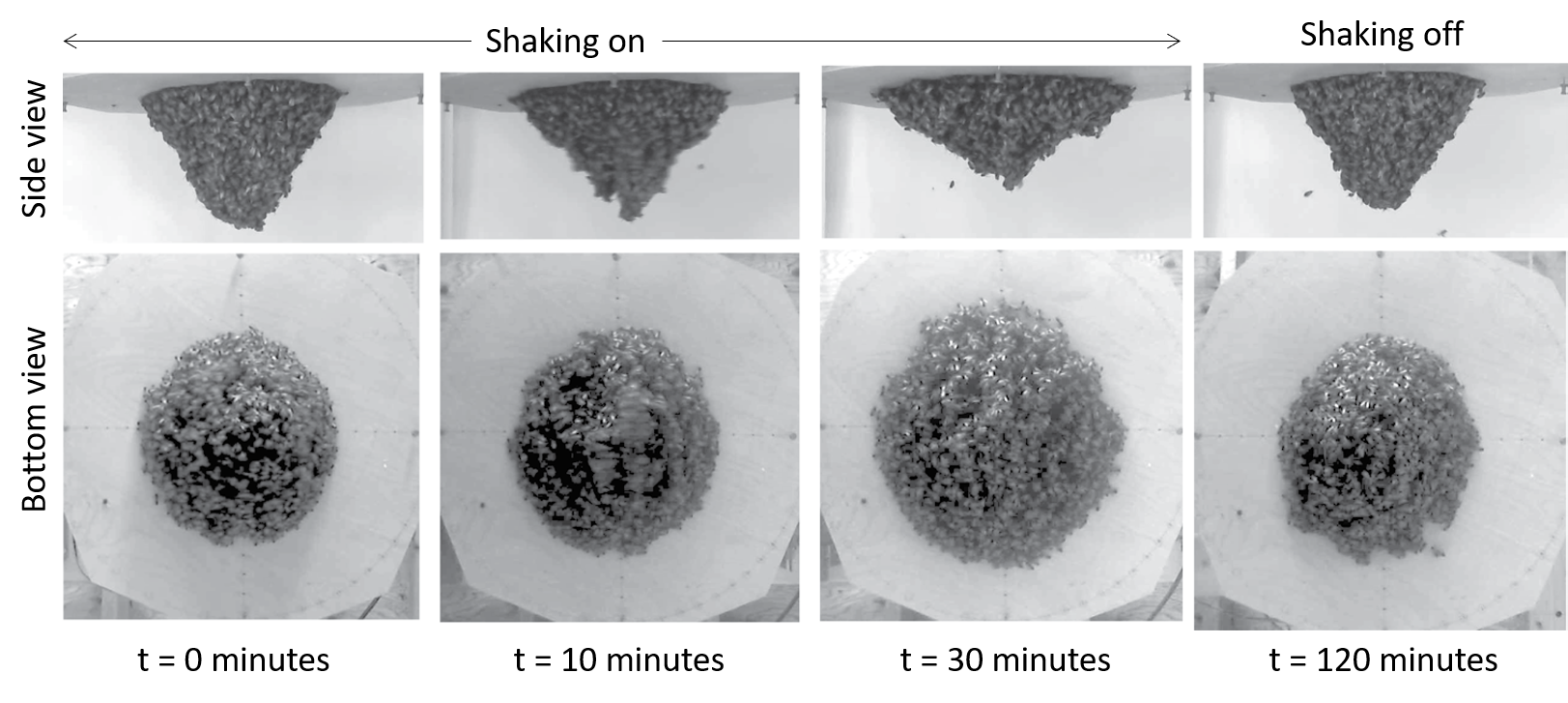
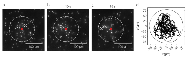
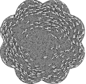
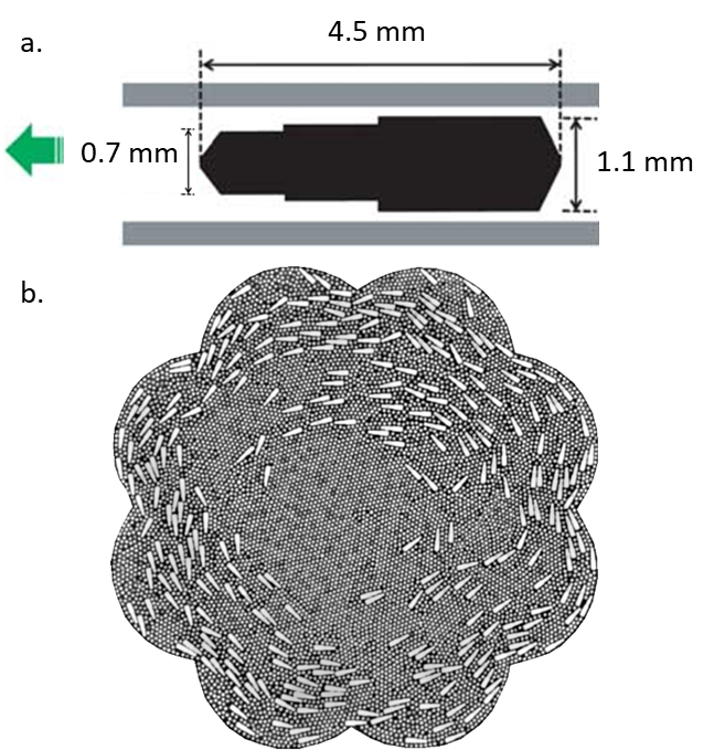
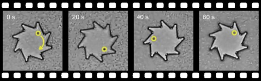
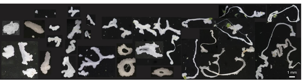
Meet Trichoplax adhaerens, a microscopic marine animal from one of the oldest known branches of the evolutionary tree. It looks like a microscopic cell sandwich: two layers of epithelial cells (which make up the surfaces of our organs), with a layer of fibre cells in between. As depicted in Figure 1, T. adhaerens takes a wide variety of shapes from disks to loops to noodles and more. Oddly,  T. adhaerens ruptures when it moves around, a self-induced fracture behavior that has recently captured the attention of physicists and engineers. Fracture is the technical term describing the process by which an object breaks into distinct pieces due to stress. These animals push their epithelial tissue to the breaking point, forming incredible and extreme shapes before separating altogether. This is a surprising behavior for epithelia, which usually prefer to maintain their integrity.  By modeling how T. adhaerens rips itself apart when moving, we can improve our understanding of how soft materials and especially biological tissues behave on the verge of breaking.

Prakash, Bull, and Prakash conducted a two-pronged analysis of fracture in T. adhaerens:  live imaging to record the fracturing in real time and computational modeling to simulate the response of the tissue when stretched too far. The drastic mechanical behavior in question also motivated the researchers to perform a more general inquiry into the competition between flow and fracture in materials that are dramatically deformed relatively quickly. Flow is like stretching out a piece of chewing gum, whereas fracture is like snapping the gum in two. The computational model proposed by the authors helped paint a clearer picture of what happens when T. adhaerens rips apart.

Figure 2: Model tissue is described as a collection of balls and springs. Balls represent cells, and springs represent the sticky adhesion between cells. Springs apply restorative forces to the cells, but can break if stretched too far. This model was used to study the ventral (bottom) epithelial layer, which consists of epithelial cells (green) and larger lipophil cells (red). Figure courtesy of the original article (Extended Data).

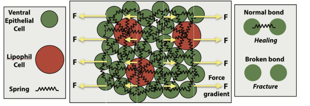
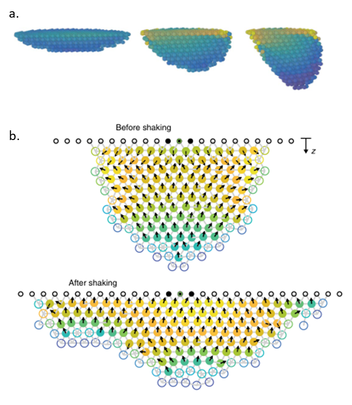
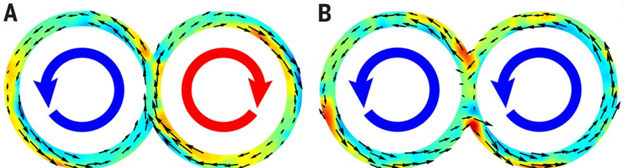
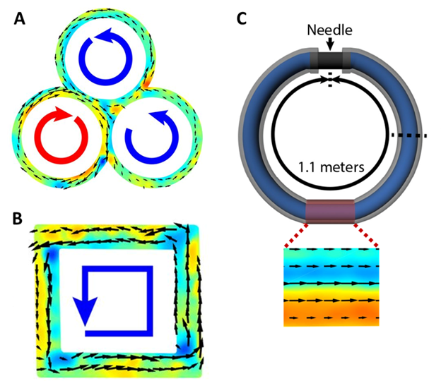
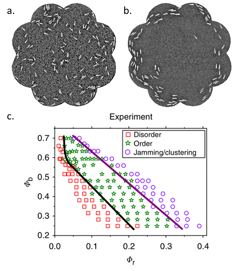
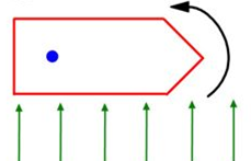
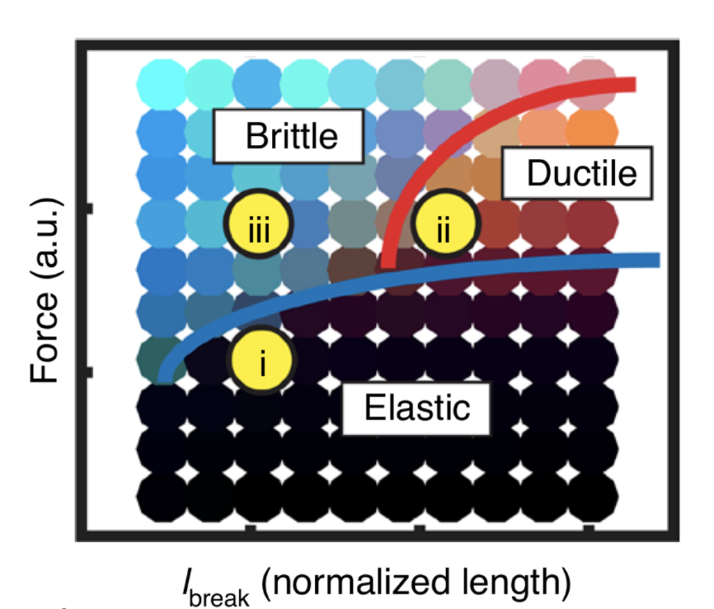
The computational model that the researchers used is based on a sticky ball and spring model, as shown in Figure 2, where each ball represents a cell and each spring represents the sticky junctions that cells use to adhere to one another.  The springs break if the balls move too far away from each other, which represents cells being unstuck from their neighbors.  Two cell types are represented in the model epithelial layer in Figure 2: epithelial cells, which are small and comprise the bulk of the tissue, and lipophil cells, which are larger and less common.  Using this model for living tissue, the authors conducted computational simulations where the tissue was stretched to a breaking point. They found that there are three possible tissue behaviors that depend on the strength of the driving force applied to the simulated tissue. For weak forcing (low stress), the tissue behaved elastically and so responded in such a way that it could recover its original shape. For intermediate forcing (medium stress), the tissue underwent a “yielding transition” where the material transitioned from elastic response to plastic response. During plastic response, permanent distortions occurred in the material, and the material could not recover its original shape. In this case, the tissue is ductile and undergoes local changes, like cells interchanging with neighboring cells, to relax some of the pent-up stress. For stronger forcing (high stress), the tissue undergoes brittle fracture where the bonds between cells break with little opportunity for relaxation. The three behaviors in the model represent a transition from elastic to ductile to brittle responses. Using this model of tissue response to applied force, the authors mapped the conditions that lead to different tissue behaviors, as sketched in Figure 3.

Figure 3: Tissue phase diagram (elastic-ductile-brittle) generated by the tissue simulations. The elastic regime (i) implies that bonds do not break, and neighbors are not exchanged. Above the yield transition (blue line), cells undergo local relaxations and flow in the ductile yielding regime. To the left of the red line, cell bonds tend to break and form gaps between cells, demarcating the brittle fracture regime.  Figure courtesy of the original article.

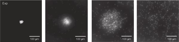
Guided by a better understanding of tissue mechanics thanks to the computer model, the authors experimentally measured the brittle and ductile responses in T. adhaerens. They found that both material responses can occur in our microscopic friend. The ability to access both regimes is important because the ductile response yields by flowing (helping form the longer shapes in T. adhaerens) whereas the fracture response accounts for asexual reproduction by splitting into two separate new individuals. The authors’ combined approach of experimental data that motivated the development of a computer model, which in turn guided further experimental inquiry, is an important modern scientific paradigm. Both approaches are incredibly important tools in the biological and soft matter sciences’ toolkit. Joint application of these tools lets us draw general conclusions from specific experiments as well as apply those general conclusions back to answer specific questions – like explaining how T. adhaerens achieves the diversity of shapes in Figure 1 and how this relates to its hardiness and evolutionary goal of reproduction.  Further, the epithelial layer computational modeling technique generalizes this tissue mechanics study to help us describe fracture versus flow in any living tissue, including our own.

Who needs polymer physics when you can get worms drunk instead?

Original paper: Rheology of Entangled Active Polymer-Like T. Tubifex Worms (arXiv here)


If you speak to a soft matter physicist these days, within a few minutes the term “active matter” is bound to come up. A material is considered “active” when it burns energy to produce work, just like all sorts of molecular motors, proteins, and enzymes do inside your body. In this study, the scientists are focusing specifically on active polymers. These are long molecules which can burn energy to do physical work. Much of biological active matter is in the form of polymers (DNA or actin-myosin systems for example), and understanding them better would give direct insight into biophysics of all kinds. But polymers are microscopic objects with complex interactions, making them difficult to manipulate directly. To make matters worse, physicists have yet to fundamentally understand the behaviors of active materials, since they do not fit into our existing theories of so-called “passive” systems. In this study, Deblais and colleagues decided to entirely circumvent this problem by working with a much larger and easier-to-study system that behaves similarly to a polymer solution: a mixture of squirming worms in water.

The researchers focused on the viscous properties of this living material, which behaves somewhat like a fluid. Viscosity is a measure of a fluid’s resistance to gradients in the flow. Polymer fluids are highly viscous because the long molecules in a polymeric liquid get tangled up in one another. Physical descriptions of most fluids assume that viscosity is a constant (so called Newtonian fluids), but many materials exhibit what is called shear thinning. This is when a fluid flows more easily as one applies an increasing shear force, that is, a force pulling the system apart. We encounter shear thinning at the dinner table all the time when struggling to pour ketchup, another polymeric fluid, out of a bottle. If the bottle is shaken fast enough, increasing the shear force applied, the ketchup flows smoothly like a liquid. In polymer systems (like xanthan gum in the ketchup) shear thinning happens when polymers are pulled apart fast enough that they tend to align together, which loosens the entanglements that held the system together before. 

In this study, the researchers asked: how does shear thinning behavior change if the polymers in question were alive? To answer this question, they set out to measure the shear thinning properties of a mixture of worms at various levels of worm activity. Here, “worm activity” refers to how fast the worm is wriggling, which is calculated by measuring how quickly the distance between the two ends of a given worm changes. This leads to two logistical questions: how is the level of worm activity being modified, and how is the viscosity being measured?

Figure 1. This movie shows two worms, one in water (left) and one in a water + alcohol mixture (right). The worm on the right shows a decrease in activity when they are exposed to alcohol, which is one of the two ways the researchers modified worm activity in this study. Video taken from the original article.

The answer to the first question should be familiar to many humans. To make the worms less active, they were put into a solution containing water and a small amount of ethanol, the same type of alcohol found in beer, wine, and spirits. Once the worms were nice and drunk, the researchers noticed that they squirmed about more slowly, as shown in Figure 1. Thankfully, when the ethanol was removed, the worms returned to their previous level of activity! To make sure the alcohol wasn’t doing anything funny to the worms, they found a second way to reduce the activity — by reducing the temperature of the worm solution. Colder temperatures made for more chilled out worms, no pun intended.

Figure 2. This movie shows the functioning of the rheometer. The worms are placed inside a chamber between two plates. The top plate rotates with respect to the bottom plate, and the response of the material is measured. Video taken from the original article.

The researchers used a device called a parallel-plate rheometer to understand the shear thinning behavior of this living polymer system. As seen in Figure 2, a parallel-plate rheometer sandwiches a sample in between two flat plates and viscosity is measured by determining how much force is necessary to rotate the top plate, effectively pushing the material by twisting its surface. The viscosity of the worm mixtures was first determined at three different temperatures, and for worms drunk on ethanol. The results were surprising! The rheological behaviour of the low-activity worm mixtures matched with theories of polymer shear thinning quite well. It seems the worms have the same alignment properties as passive polymer solutions under shear!

So what happens when the worms are sober, more active, and wriggling around? They saw that the required twisting rate needed to thin the mixture decreased. In this case, the worm activity allowed for easier and quicker rearrangement while the mixture was pulled apart by the rheometer’s twisting motion. One can imagine that instead of needing to pull all the worms to the point of alignment, it may have been enough to nudge them in that direction and their wriggling did the rest. We can now imagine that the same thing might be true for non-living polymers: if a polymer material with shear thinning behavior is given an extra source of activity, then its thinning behavior may become more significant. 

The lesson to be learned here is partly about worms, polymers, and the adverse effects of ethanol, but really this experiment is a testament to the power and generality of physical descriptions. This study teaches us about the possible behavior of an active polymer system with processes that are relevant on the scale of a few micrometers, by studying real life worms that you can see with the naked eye! In general, it is usually possible to find analog systems that have the desired properties for your study, but which are easier to manipulate. Physics then gives you the bridge between the system of interest and your simpler analog, allowing you to harness the power of interdisciplinary science to ask questions previously unanswerable.

Featured image for the article is taken from the original article.

Huddling penguins make waves in the Antarctic winter

Original article: Coordinated Movements Prevent Jamming in an Emperor Penguin Huddle

Standing in the center of a crowded bus on your way to class, you might think: “why don’t these people just move? It’s hot and I can’t breathe!” Male penguins huddling to keep their eggs warm in the Antarctic winter have the opposite problem – no penguin wants to be at the cold edge of the huddle. A penguin in the huddle wants to stay in the warm center, since the outside temperature can reach -45 oC. However, penguins on the edge of the huddle are trying to push through the crowd to reach the center. Through the independent motion of each penguin, the huddle stays tight enough for the center to remain warm but loose enough to keep moving.

In today’s study, Zitterbart and colleagues investigate how huddling Emperor penguins can keep moving, as in this video.  They find that individuals take small, coordinated steps that reorganize the huddle on a time scale of hours.

Zitterbard and colleagues film a 2000-penguin colony (shown in Figure 1a) for 4 hours and track the positions of the penguins, with an x-coordinate corresponding to horizontal position on the camera image and  y-coordinate corresponding to the vertical position on the camera image. When huddling, the penguins all face in the same direction and are arranged roughly in a hexagonal grid. Every 30 to 60 seconds, the penguins take small steps, 5-10 cm long. Figure 1b shows the track of one penguin, with a point every 1.3 seconds. There are clusters of points where the penguin is standing still (with no significant change in position), and then a straight line when the penguin takes a step.

Since penguins at one spot in the huddle don’t know that another part of the huddle is moving, they don’t all step at once. Instead, there is a wave of moving penguins that moves through the huddle at a speed of 12 cm/s, like a sound wave traveling through a material. Figure 1c shows the tracks of several penguins at the same y-position and different x-positions in the huddle. Their horizontal motion is correlated – the penguin at the top track moves first, and then the motion propagates to the neighboring penguins as a wave. 

Figure 1. a. A photograph of huddling penguins with x- and y- coordinate axes. b. A track of a single penguin with points every 1.3 seconds. Clusters of points mean the penguin isn’t moving, and a straight line means the penguin took a step. c. Horizontal motion of several penguins. These penguins are at the same vertical position in the huddle but different horizontal positions. The slope represents the 12 cm/s motion of the wave of moving penguins.

An unusual aspect of this study is that the results section is short – the authors only report the traveling wave of penguins through the huddle. However, they then move to an explanation of penguin motion using very interesting  analogies to granular materials (such as sand or coffee beans). 

There are three effects of the small steps:

  1. They allow the penguins to reach the best density for warmth.
  2. They move the entire huddle forward, and merge small huddles into big ones.
  3. They reorganize the huddle, allowing penguins to leave the huddle at the front and join it at the back.

The combination of small penguin movements and organized huddling is similar to the way colloids [1] solidify when the particles in the colloid attract one another. Penguins huddle when they are “attracted” to each other by cold temperatures; colloids are attracted by electrostatic or intermolecular van der Waals forces. Thinking of a group of organisms as a fluid, such as smoothly flowing fish schools and turbulent bacteria, is a well known method for understanding their behavior. In contrast, the small steps in a dense group of penguins is reminiscent of a material going from a fluid to a solid state. The waves in the huddle are similar to waves in other groups of animals, like human crowds rushing to escape a room. Luckily, the penguin waves do not result in injury. (Usually.)

Through small, careful steps, penguins are able to create a solid cluster of warmth in the Antarctic winter. If we took a hint from the penguins and were more careful about our motion when on a crowded subway, maybe our commutes would be much more pleasant experiences. Of course, the huddling penguins are not bounded by the walls of a bus – how they would move if they didn’t have an open boundary is still a mystery!


[1] Mixtures of small particles dispersed throughout another substance, such as the fat suspended in a water solution to form milk.

The dance of swarming flies

Original article: Emergent dynamics of laboratory insect swarms

Imagine yourself as a small fly called a midge (shown in Figure 1a). You used to live in a lake as a small larva with no concerns in life except swimming, eating, and growing. One day, you hid underwater and formed a cocoon around your body as it developed wings, legs, and antennae. A few days later, you swam to the surface and burst out of your cocoon as an adult fly — a male. As a new adult male, you find the clock ticking – you have only a few days to find a mate before you die.

Attracting a female is difficult for a tiny midge – how is she going to see you flying around? Fortunately, you can team up with hundreds of other male midges. Together, you fly above the lake in a stationary swarm that looks like a large cloud. Females can find this swarm and fly into it for their choice of mate. 

In today’s study, Douglas Kelley and Nicholas Ouellette investigate how the motion of midges in a swarm helps the swarm stick together.

Figure 1. (a) A midge is a tiny fly that forms mating swarms above lakes (image from Wikipedia). (b) Midges tracked in a swarm in the laboratory, with different midges in different colors (Figure adapted from original article)

The researchers set up midge swarms in the laboratory and film them with three infrared cameras. They track all of the individual midges in the swarm and calculate their trajectories. Tracking dozens of small midges is not easy! First, they use the 2D images from the three cameras to locate the flies in 3D for each frame. Then, they use a technique originally developed for studying turbulent fluid flows to generate the trajectories over time. This technique uses the history of each midge to estimate where it is likely to be next and looks for midges in that area at the next time step. The resulting trajectories are shown in Figure 1b.  The positions, velocities, and accelerations of the midges give clues about how the swarm moves.

First, Kelley and Ouellette discuss the position of the midges. They plot the logarithm of the probability (log_{10} P) of finding a midge in a point in the swarm in three dimensions in Figure 2. Bright red represents a high probability of finding a midge, and blue represents a very low probability. Midge swarms are nearly symmetric, but larger swarms (of 100 individuals or more) are slightly taller than they are wide. This is unlike bird flocks, which are nearly two-dimensional.

Figure 2. Probability of finding a midge at x, y, and z coordinates in the swarm. Bright red colors indicate high likelihood of finding a midge, and blue represents a very low chance of finding a midge in that position. (Figure adapted from original article)

The researchers then investigate the velocities of the midges. Since the swarm is stationary, the average velocity of all the midges in the swarm is nearly zero. It turns out that the standard deviation, or the variation, of the velocities of the individual midges is more useful for understanding the motion inside the swarm. Midges fly twice as fast horizontally as vertically, just like birds in a flock. However, unlike flocks of birds, the midge swarms  are not polarized — a midge does not tend to fly in the same direction as its neighbors. Finally, Kelley and Ouellette investigate the acceleration of the midges in the swarm. The midges are equally likely to turn in any direction, unlike birds or fish. Relative to their body size, larger animals have more inertia than smaller ones, and must exert a lot more effort to turn, accelerate, and decelerate. Thus, they tend to keep moving in the direction they are currently moving. Midges, on the other hand, can turn and easily move in any direction. Kelley and Ouellette find the average acceleration of the midges in the swarm in the x-direction as a function of the midge’s x-position, \langle a_x|x \rangle, in Figure 3.  The midges tend to accelerate towards the center of the swarm, keeping the entire swarm together despite the midges’ constant motion. [1]

Figure 3. Acceleration of the midges in the x-direction as a function of the x-position for several midge swarms.  Each line represents a different swarm. When a midge is at the right edge of the swarm, it accelerates to the left (and vice versa).  (Figure adapted from original article)

In this study, Kelley and Ouellette quantify a new type of swarming behavior. Unlike most other animal aggregations like bird flocks and fish schools, midge swarms stay in one place, helping female midges find the love of their very short lives.


[1]  Surprisingly, when Kelley and Ouellette investigated the mean square displacement of the midges, they found that the midges act as if they are trapped in a box with walls.

Cell migration: a tug-of-war inside your body

Original article: Physical forces during collective cell migration

If you ever played tug-of-war in elementary school, you might remember that it isn’t the friendliest game. People fall over, hands get burned from holding on to the rope, and knees get scraped from falling on the ground. Although victory can be sweet, the injuries that come with it may make you never want to play the game again. Perhaps surprisingly, there is a similar ‘’tug-of-war” happening inside your body, as individual cells move around from one place to another in a process called cell migration. What’s more, this microscopic tug-of-war may help to heal those scrapes and bruises that happened in elementary school, and those that happen in your everyday life.

A single cell moves by detaching and reattaching from the substrate, or the surface it is on, as the cell  expands and contracts. This movement exerts forces on the substrate. (These forces can actually be measured directly –  this is the topic of a previous softbites post.) When many cells move together in a “cell sheet”,  their motion becomes more complicated. Not only do cells push and pull on the substrate, but they also push and pull on the cells that surround them.  In today’s study, Xavier Trepat and colleagues show that there is a “tug-of-war” between cells that causes them to migrate.

Previously, it was thought that only the cells at the very front of the mass of migrating cell, or the leading edge of the cell sheet, exert forces on the substrate. According to this picture, most of the cells get passively pulled along by the leading edge, and neither push nor pull on the substrate. By measuring the forces the cells exert on the substrate, Trepat and his colleagues discovered that, in fact, all of the cells are involved in pushing the cell sheet forward.

The researchers measured the forces in a moving sheet of cells, taken from canine kidneys, growing on a gel substrate using a technique called traction force microscopy. The first step of this technique is to track the displacements of different points within the substrate as the cells move. Then, the mechanical properties of the gel are used to calculate the forces on the substrate generated by this motion. The researchers mapped the value of these forces using different colors, with red and blue representing very strong forces and black representing zero force. They first looked at what happened at the leading edge of the cell sheet, as in Figure 1.


Figure 1. a. Image of the cell sheet, in which individual cells are outlined in white. The field of view is 700 microns by 700 microns. b. The forces that the cells exert perpendicular to the leading edge of the cell sheet. c. The forces that the cells exert parallel to the edge of the cell sheet. Bright red and blue colors indicate strong forces (up to 100 Pa of stress), while black color indicates low forces. (Images adapted from the original article.) The cell sheet’s expansion was recorded in a video as well.

The researchers separated the normal forces (Figure 1b) — those exerted by the cells perpendicular to the leading edge of the cell sheet, or in the direction of the cells’ motion — from the forces exerted parallel to the leading edge of the cell sheet (Figure 1c). The bright red and blue colors in Figure 1 show that cells well inside the cell sheet exert forces on the substrate. From this, they hypothesized that instead of having “follower” and “leader” cells, all the cells contribute into pushing and pulling the cell sheet as they move.

The researchers then looked at larger areas of the cell sheet, such as that  shown in Figure 2. The bright colors near the edges correspond to strong forces,  while the black spots show that the forces in the center of the cell sheet are weaker. This suggests that the cell sheet “tugs” both to the right and the left as it expands. As the cells exert forces on the substrate, they exert forces on each other. The cells pulling to the right and the left are similar to two teams pulling a rope in a game of tug of war. The sheet of cells is like a rope that grows in the direction of the tugging of the cells.

Figure 2. Forces exerted by a larger piece of the cell sheet. Bright red indicates strong positive forces and blue indicates strong negative forces, while black indicates low forces. The scale bar on the bottom right is 200 micrometers.  (Image adapted from the original article.)

Next, the researchers wanted to understand how being tugged on by its neighbors affects the motion of individual cells: does the tug of war consistently pull a cell in a particular direction? Or is the cell equally likely to be pulled in any direction?  To answer this question, Trepat and colleagues measured the average force exerted on a cell by its neighbors, as a function of the distance of that cell from the edge of the sheet. If each cell was moving independently, the average normal force inside the sheet would be zero – on average, no cell would be pushing or pulling any other cell to a specific direction. Instead, as shown in Figure 3, the average force was not zero, and was actually higher for distances farther from the sheet’s leading edge. In other words, the cell sheet is expanding from the inside more than it’s being pulled from the edge.


Figure 3. The average normal force exerted on a cell by its neighbors, \sigma_{xx}, is higher farther from the leading edge of the cell sheet. (Figure adapted from the original article.)

Each individual cell crawling on a substrate has little effect on its surroundings, but many cells acting together can exert forces on each other to guide the collective in a particular direction. As cells replicate, such as in a healing wound, this guiding helps the cells expand in directions where there is space to be filled. This study by Trepat and colleagues reveals for the first time the tug-of-war that allows the tissues in our bodies to grow and heal.

Sticky bees: How honeybee colonies stay safe outside their hives.

Original article: Collective mechanical adaptation of honeybee swarms


A honeybee colony can only exist when many individual bees cooperate. When a hive becomes too crowded, about 10,000 of the workers and a queen leave the hive to form their own colony. While the scout bees are searching for a new nest site, the rest of the bees are exposed to all of the dangers of the outside world, such as predators and storms, and have to stick together for protection. They form a “cluster”, which hangs on a nearby tree branch (as in Figure 1a) until a new suitable nest site is found. Sometimes, beekeepers hang these clusters from their faces as a “bee beard”.

In this study, Orit Peleg and colleagues investigated how these bee clusters stick together against the forces of gravity and the wind by shaking them and tracking how the shape of the cluster changed. Their experimental setup consisted of a board attached to a motor that shook it horizontally at frequencies between 0.5 and 5 Hz and accelerations up to 0.1 times gravitational acceleration. Peleg and colleagues put a queen bee in a cage attached to the board, leading the rest of colony to cluster around her, as shown in Figure 1b. Once the cluster formed, the researchers turned on the shaking and filmed how the bees behaved.

6-1
Figure 1. a) A bee cluster in the wild. The worker bees are protecting the queen until they find a new hive. b) A bee cluster in the lab, with the queen attached to the top board in a cage. Figure adapted from original article.

As the bee cluster was shaken horizontally, its tip swung from side to side at about 1 Hz, or one cycle per second. Peleg and colleagues tracked the bees moving from the tip of the cluster to the base as the cluster flattened over about 30 minutes. A flatter cluster does not swing nearly as much as an elongated one.  Once the shaking was turned off, the cluster elongated again after 30 minutes to two hours, longer than it took the cluster to flatten. This is shown in Figure 2.

6-2
Figure 2. A honeybee cluster adapting to shaking filmed from the side and the bottom over time. While the shaking is on, the cluster spreads out along the base, and becomes shorter. When shaking is turned off, it returns to its original form. Figure adapted from original article.

Peleg and colleagues observed that individual bees responded to the variations in strain near them. At the base of the cluster, the strain was high, since the base bore the load of the entire swinging cluster. The bees at the base stretched their limbs to hold the rest of the cluster as it swung back and forth. The strain at the tip of the cluster was lower, since the bees there did not have to stretch as much to hold on. As more bees reached the base of the cluster, it flattened, making it swing less and decreasing the local strain on all the bees. The cluster was much flatter after 30 minutes of shaking, as in Figure 2. The bees at the base then didn’t have to stretch as much to hold on, and the cluster was safe from being torn apart.  Even though an individual bee moved towards a greater strain, which may have been less comfortable for it, this collective bee behavior ultimately decreased the strain on the entire colony.

The researchers hypothesized that when a bee experienced a “critical strain”, a high value that might endanger the cluster, it moved to where the strain was higher — up towards the base —changing the cluster’s shape. To show that moving in the direction of increasing strain is a possible explanation for how the cluster flattens, Peleg and colleagues simulated honeybee clusters of different shapes under horizontal shaking (Figure 3). Each bee was modeled as a spherical particle experiencing gravity and attraction to neighboring bees. The simulated bees could not overlap with each other.

For their first simulation, the researchers simulated an entire cluster in 3D with stationary bees subject to horizontal shaking. They wanted to investigate the relationship between cluster shape and the strain.  In this simulation, longer bee clusters experienced a higher strain when they were shaken, as shown by the color gradient in Figure 3a, with yellow corresponding to a higher strain than blue.

A second set of simulations allowed bees to break their connections with their neighbors and move in the direction of increasing strain if their neighboring strain was above a critical value. As expected, bees moved towards the base when shaking was simulated, and the cluster flattened out forming a shape similar to what was observed with real bees in Figure 2, shown in Figure 3b.

6-3
Figure 3. a) Three clusters simulated with horizontal shaking, from flat to elongated. Longer clusters have much stronger strains at the base. Blue colors correspond to lower strains while yellow corresponds to high strain. b) When shaking is turned on, simulated bees move towards higher strain (in the direction of the arrows) and flatten the cluster. Red and yellow colors correspond to higher strains. Figure adapted from original article.

This behavior lets bees keep the queen safe and the colony together on the tree when the cluster swings side-to-side in the wind. The cooperation of bees following simple rules lets the colony survive until it finds a new home.

Using sound to build a wall: how physicists measure pressure in active systems

Original paper: Acoustic trapping of active matter


You know how sometimes you tell to yourself things like “life is complicated”? Theoretical physicists are constantly reminded of this fact when studying living organisms. Recently, a new field of physics has emerged, inspired by the observation of living systems. What forces do cells exert during metastasis in cancer? What are the growth dynamics of biofilms of bacteria? How can a school of fish organize itself and move simultaneously? These are questions raised in the physics of active matter. Active matter is an assembly of objects able to move freely and capable of organizing into complex structures by consuming energy from their environment. Active matter can be composed of living or artificial self-propelled particles.

However, active systems differ from a simple gas or liquid because they are out-of-equilibrium. A system is in equilibrium if there is an energy balance between the system and the environment. When the energy isn’t balanced, the system will evolve toward an equilibrium state. Imagine a ball on a hilltop: it is in an out-of-equilibrium state until it has rolled down and stopped at bottom of the hillside. Now imagine that the ball is an active particle. This means it can consume energy from its environment to propel itself back up the hill, which drives the system out of equilibrium.
But physical notions such as pressure or temperature, are defined in thermodynamics only at equilibrium. This is why bridging the gap between physics and active matter has been a new challenge for theoretical physicists. Today’s paper focuses on the definition of a new quantity called swim pressure and highlights how researchers achieved its experimental measurements using an acoustic trap.

Rather than dealing with living organisms in this study, Sho and his collaborators used a system of artificial self-propelled particles, called Janus particles. They are made of two half faces; one in polystyrene and one in platinum [1]. Once immersed in a liquid, the platinum coating reacts with hydrogen peroxide contained in the liquid. The available energy resulting from this chemical reaction is then converted into motion. Particles move individually and randomly (analogous to an atom’s motion in a gas).

Due to self-propelled motion, active particles exert a mechanical force on their surrounding boundaries. In other words, a particle would naturally swim away in space unless confined by walls. The pressure exerted by active particles on the walls that confine them is the swim pressure. This is analogous to the definition of pressure from a microscopic point of view, which is the result of atoms colliding on a surface. Now that the theory is set, researchers try to measure swim pressure experimentally. But to control, confine and observe micro-particles between walls that you can remove at will is quite a challenge.

nodes
Figure 1. The curves represent two profile of an acoustic wave throughout time. Particles migrate to nodes due to the difference in acoustic pressure between nodes and antinodes.

Sho and his collaborators at California Institute of Technology did not actually use physical walls in their experiment but instead used sound. When an acoustic wave propagates through a material, the deformation of the material causes a local pressure. Using this acoustic pressure, researchers can move objects between specific locations called nodes, which are special locations where the pressure wave is stable in time. The local pressure is minimal at nodes, while pressure is maximal at antinodes (see Figure 1). Since objects move from high to low pressure, the particles become trapped at nodes (see Figure 1). This technique is called an acoustic tweezer, or acoustic trap. Here, researchers built an acoustic trap such that many particles are confined over a large trap area.

figure1
Figure 2: a-c. Snapshot of Janus particles in an acoustic trap (watch movie here). The red spot is the center of the trap and the white dashed line represents the contour of the acoustic trap. d. The figure shows trajectories of Janus particles moving randomly inside the trap (images adapted from Sho and coworkers’ original paper).

The researchers also adjust the size and force of the trap as a function of the velocity of active particles. Over time, more particles get trapped, and a densely packed cluster forms (see Figure 2). Particles can move within the trap area, but cannot exit (see Figure 2d). Then, when the acoustic tweezers are turned off, the cluster explodes! Meaning that free from confinement, active particles spontaneously disperse (see Figure 3). Thus, knowing the acoustic pressure and measuring the dispersion of particles over time allows researchers to measure the swim pressure.

figure2
Figure 3. Snapshots of Janus particles at different times after the acoustic trap has been released (watch movie here). The active cluster explodes, resulting in Janus particle dispersion (Images adapted from Sho and coworkers’ original paper).

When you inflate a soccer ball with a pump, the walls will experience more collisions with the air molecules, meaning pressure increases. Similarly, squeezing the ball reduces space between the molecules and also results in an increase in pressure. These types of pressure changes are analogous to those observed in Sho and collaborators’ experiments. As shown in Figure 4, swim pressure increases over time as more particles get trapped (like pumping air into the soccer ball). Swim pressure also gets stronger for smaller trap area (like squeezing the soccer ball). But despite the analogy, we must not overlook the complexity behind the physics. Swim pressure is different from the pressure we experience every day, which comes from atoms and molecules. Here the classical model of pressure is an inspiration to build a new model. And as Figure 4 illustrates, the theory is consistent with experimental observations and validates this concept of swim pressure.

figure3
Figure 4. Evolution of the swim pressure as a function of time for two different size area. The swim pressure is higher for smaller trap areas. Researchers compare here experimental data with numerical simulations and theory (adapted from Sho and coworkers’ paper).

To conclude, today’s paper shows how classical physics quantities can be redefined to describe a new phenomenon in active matter. Sho and his collaborators used an ingenious device to measure the swim pressure exerted by active particles for different degrees of confinement and different crystal size. Their results confirm experimentally the theory of swim pressure established in a new approach of active matter, and open ways to a better description of the living world (from molecular to cells dynamics, bio-films formation, collective motion…). So indeed, life might be complicated, but from the point of view of scientists, this is what keeps them excited.

[1] these particles were named Janus particles in reference to the Hall-faced Roman God Janus.

Tiny Tubes Racing in a Donut-Shaped Track

Original paper: Transition from turbulent to coherent flows in confined three-dimensional active fluids


The shape of a container can affect the flow of the fluid inside it. Water in a narrow stream flows smoothly, but once the water molecules make their way into a pond, they spread out and no longer flow coherently. If you blow into a long, narrow straw, the air will go straight through. Once the air flows into the large room you are standing in, it slows down as it mixes with the air around it, so someone standing five feet away from you won’t feel a breeze at all.

The above examples show how the shape of a container affects the flow of passive fluids. In today’s study, Kun-Ta Wu and colleagues investigated how the motion of active fluids, fluids that flow using an internal source of energy, is also affected by the shape of their container. They used a system of microtubules, chains of proteins assembled into long, stiff rods. Clusters of a protein called kinesin exert a force on microtubules by “walking” along them. Microtubules interact with each other to form swarms or turbulent-like flows.

Wu and colleagues created 3D toroidal racetracks with rectangular cross-sections to confine the microtubule bundles. They saw coherent flows in racetracks with square cross-sections, but if the channels got either too thin and wide or too tall and narrow, the flow became turbulent (Figure 1). This result is described in this Softbites post from last year.

5-1
Figure 1: Comparison of coherent and turbulent flows around a track. The left side of each track shows the motion in an instant, while the right side shows the average motion over a long time. The color represents the local direction of spinning and the black arrows indicate the direction of motion. Microtubules in a red spot are spinning clockwise, those in a yellow spot are not spinning, and those in a blue spot are spinning counterclockwise. Image adapted from original article.

After Wu and colleagues got microtubules to flow by themselves, they placed them in increasingly complicated tracks. Active flows happened in any closed loop with an approximately square cross-section. Microtubule flows solved a maze, as in Figure 2, by flowing through the connected straight and curved sections, but not sections leading to dead ends. The dead ends slowed down the flow in the connected sections to about half the speed of a toroidal racetrack with an equivalent length.

5-2
Figure 2: Microtubules flow in straight and curved sections of the maze in closed loop, and no net flow loop in sections leading to dead ends. Black arrows show the direction of the flow and colorful arrows point to sections at which mean flows are measured. Figure adapted from original article.

Wu and colleagues then created tracks made out of overlapping tori, or donuts. In the tori, microtubules spontaneously flowed in the same or in different directions, as in Figure 3. When the active flow was clockwise in one torus and counterclockwise in the other, the direction of flow in the overlap was the same, and the flow kept going (A). When they were both counterclockwise, two flows came into the overlap in opposite directions, and there was no flow in between the tori (B). Watch a video of this here.

5-3
Figure 3: Microtubules can flow in connected tori in (A) the same direction and (B) opposite directions. Figure adapted from original article.

Microtubules created an active flow when a third torus was added (Figure 4A). They also navigated a square racetrack, although the corners created small vortices and slowed them down (Figure 4B). Finally, microtubules still flowed in a very long torus made out of a 1.1 meter-long tube joined at the ends by a needle (Figure 3C).

5-4
Figure 4: (A) Flows in 3 overlapping tori. (B) Microtubules flow around a square racetrack in the direction of the blue arrow. (C) Microtubules even flowed around a very long (1.1 meter) track. The closeup shows a time-averaged flow inside a small section of the tube. Figure adapted from original article.


Thus, these flows of microtubules aren’t just a one-time phenomenon that’s hard to replicate—no matter how much the researchers changed the system, as long as there was a closed loop with an appropriate cross-sectional aspect ratio, there was a flow.

These flows inside channels are interesting—but are they useful? The researchers suggest that a system like this could act as an internal power source for very small devices, but this application is still far in the future. It is also possible that a similar motion is used inside living cells to transport materials in a process called cytoplasmic streaming. More importantly, these flows are a beautiful example of collective motion induced by physical forces, helping scientists elucidate how swarms can form at all length scales.

Flocking rods in a sea of beads: swarms through physical interactions

Original papers: Flocking at a distance in active granular matter


Many living creatures, such as birds, sheep, and fish, make coherent flocks or swarms. Flocking animals travel together, coordinating their speed and turns in an often visually striking manner. This can have benefits for the animals – flocking birds can use aerodynamics to fly more efficiently, sheep can move together as a group to evade predators, and fish can use collective sensing to find preferred locations in their environment. Flocks emerge in biological systems because animals try to follow their neighbors.

But how about non-living things? Can they spontaneously form swarms without any biological motive?

In “Flocking at a distance in active granular matter”, Nitin Kumar and colleagues investigate how non-living rods can form flocks just like animals do. They create a flock of self-propelled rods in a sea of spheres and show how a small concentration of these rods can transport a large load of passive spheres.

In this study, the active agents are cone-shaped brass rods, as in Figure 1a, that move through a layer of aluminum beads. The rods and beads are placed in a flower-shaped dish, as shown in Figure 1b, and covered by a glass lid. The surface vibrates, making the rods bounce up and down. Friction between the floor and ceiling propels a rod in the direction of its tip. Thus, each otherwise immobile rod moves by itself. Because the rod shape isn’t perfect, it turns a little with each movement, and randomly wanders around the surface.

4-1
Figure 1: (a) Schematic of a cone-shaped rod. (b) Experimental setup of brass rods moving through aluminum beads. The flower shape is used to prevent rod clumping at the walls. Figure adapted from the original article.


At low concentrations of both rods and beads, the rods wander around randomly and independently of one another. Past some critical concentration of either, however, the rods suddenly align and swarm around the surface in a random direction. Once the rods begin swarming clockwise or counterclockwise, they do not change which way they swarm.

A comparison of randomly moving and aligned rods is shown in Figures 2a and 2b. The motile rods drag the inactive beads alongside them. The flow of the beads then reorients rods throughout the surface, until the rods are aligned. This is similar to what happens in biological flocks, where each animal tries to follow their nearest neighbors. Small turns of individuals turn the entire flock, forming beautiful patterns.

The researchers created a “phase diagram” of rod and bead concentrations in the experiment (Figure 2c). At rod and bead concentrations below the black line, the rods move randomly. When either rod or bead concentration is increased, swirling begins. Increasing the number of rods increases the number of agents that can interact with each other. Increasing the number of beads increases the density of material through which the rod forces propagate. Finally, if the concentrations are too high, the system becomes jammed, and the rods can’t move enough to align in the first place.

4-2
Figure 2: (a) Randomly moving rods. (b) Aligned rods swirling in the same direction. (c) Phase diagram showing transitions between the different behaviors of the rods and beads depending on how concentrated they are. Image adapted from the original article.

So far we’ve just discussed the motion of the rods. But what about the beads themselves? The flocking rods push them in a coherent pattern, the velocity field of which is shown in Figure 3. The rods don’t just align – they also affect their surroundings, and transport the beads as cargo.

4-3
Figure 3: Velocity field of beads that are pushed around by swirling rods.

To figure out how rods align and swarm, Kumar and colleagues developed a mathematical model for the sea of beads and rods as a “fluid” of moving beads (since there are many more beads than rods) and simulated the motion of all the rods and beads. They identified two key parameters in their equations that corresponded to:

  • Adding more rods or stronger rods results in more beads being dragged, increasing the force on each rod.
  • The “weathercock effect” affects how easily rods turn to follow the flow of the beads surrounding them. A rod with an off-center pivot (as in Figure 4) that experiences a force from the surrounding beads will turn in the direction of the forcing.

The interplay of rods pushing beads, and beads reorienting rods, form a swarm.

4-4
Figure 4: “Weathercock effect” reorients rods with an off-center pivot in the direction of the flow of the surrounding beads.

This study shows that simple mechanical interactions can cause swarms. Living creatures, such as fish and bacteria, may have taken advantage of the swarms caused by their interactions with each other to survive as they evolved.

Not Just Spinning Their Gears: Extracting Useful Work from Bacterial Swarms

Original papers: Bacterial Ratchet MotorsSwimming bacteria power microscopic gears


Imagine you and your friends are trapped by a super-villain in a cage. There is a giant gear with a diameter half the length of a football field in the center. The only way to open the cage door, get out, and stop the villain’s evil plans will be to rotate this gear by one full revolution. This is a daunting task for one person — but if you have enough friends, you can grab the gear’s teeth and push it together to escape. An analogous task is faced by flocks of tiny bacteria in today’s two featured papers. In “Bacterial ratchet motors”, Di Leonardo and colleagues discuss the mechanics of bacteria pushing a single gear, and in “Swimming bacteria power microscopic gears”, Sokolov and colleagues discuss how bacteria can interact to power more than one gear.

Two types of bacteria were used in these studies — B. Subtilis and a harmless strain of E. Coli. A single bacterium is tiny, with a pill-shaped cell body only a couple of microns in length. One bacterium has no hope of pushing a gear one hundred times its size.  It swims around in a random, “run-and-tumble” motion. During a “run” the bacterium swims straight. It then stops and “tumbles”, changing its direction randomly, and then swims straight, or “runs” for a while longer. While bacteria swimming together in large aggregations can align and make interesting flow patterns, up to now their motion has been hard to harness to provide useful work. If this technique were perfected, bacteria-powered gears could be used to power micro-devices, such as very small robots, without using an external power source.

The bacteria used in both studies swam in a liquid medium, which contained the nutrients and oxygen that they need to survive, together with one or two gears. In both of today’s articles, the gears were resting on the bottom of the liquid medium suspended above air. In Di Leonardo’s study, the drop of medium hung from a concave part of a glass slide with 48-80 micron diameter gears; in Sokolov’s study, the medium was stretched in a film between two wires with 380-micron diameter gears. The two setups are shown in Figure 1.

gear setups
Figure 1: A gear within a bacterial suspension. Di Leonardo’s setup is shown in (a), with the gear suspended above a coverslip. Sokolov’s setup is shown in (b), with the gear suspended in a film. Figures adapted from original articles.

A swarm of bacteria can’t push just any kind of gear. Di Leonardo and colleagues show that if the gear is symmetric, the bacteria can’t rotate it. In this case, there will be an equal chance of bacteria pushing on the left and the right of the gear tooth, not generating an overall rotation. To generate continuous spinning, more bacteria need to push on one side of the tooth than the other. To achieve this, the gears had asymmetric teeth, as in Figure 2a. When bacteria swim towards the corner (like the left bacterium in Figure 2a), they get stuck in the corner. The bacteria can’t escape by swimming straight, so they rotate the gear until “tumbling” and breaking free. When bacteria encounter a tooth while swimming away from the corner (like the right bacterium in Figure 2a), they swim straight off of it. This way, the gear only rotates in one direction. When several bacteria are trapped in the same corner, they spontaneously align and push the gear together, as shown in Figure 2b. This results in a larger force on the gear. The rotation of a single gear is shown in Figure 2c.

Di Leonardo results
Figure 2: Results from Di Leonardo’s paper. (a) A bacterium (represented by red rods with white heads) rotates a gear by getting stuck in a corner. Arrows represent reaction forces experienced by the gear as the bacteria hit it. The green areas and the red areas show the angle of approach when a bacterium is guided towards the corner or not. (b) Four bacteria pushing against a single tooth at the same time. (c) Bacteria spinning a gear at 1 rpm.    

Sokolov and colleagues investigated different shapes and arrangements of gears. They showed that gears with teeth either on the inside or on the outside will rotate, as in Figure 3, A-H. They then added a second gear for bacteria to spin. If two gears are close enough to each other, then their teeth ‘catch’ as in Figure 3, I and J.

Sokolov results
Figure 3: Time lapses of bacteria pushing gears with teeth on the outside (A – D), teeth on the inside (E – H), and two gears at once (I and J). Red arrows correspond to the spinning direction of the gear and black arrows point to the tracked spot on the gear. Image from original article.

Bacteria turning a gear are an example of a non-equilibrium system.  A system at equilibrium doesn’t consume any energy and doesn’t produce useful work. This might be surprising, but if a gear was placed in an equilibrium system, such as atoms in a gas, it would never rotate. An atom encountering a wall or a corner of a gear will simply bounce off, and the net torque produced by all the atoms bouncing off the gear is zero, no matter what shape it is. The difference between atoms in a gas and bacteria in a fluid is that bacteria have their own internal source of energy, and hence are not at thermodynamic equilibrium. A “running” bacterium will not just bounce off of the wall of a gear corner. Instead, its swimming will rotate the gear by the corner until the next time the bacterium “tumbles” and reorients.


Are gears rotated by bacteria actually a useful system? Sokolov and colleagues estimate that the power generated by the bacteria is 10^{-15} watts. Most electronic components, such as the ones in a cell phone, require power on the order of 10^{-6} watts. These bacteria are not — as yet — generating nearly enough power for real-world machines. Although the rotation of the gear is not powerful enough to be useful, it is amazing that such small creatures are able to do so at all.