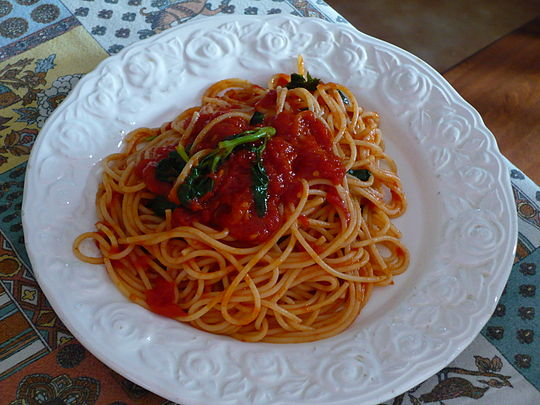
Polymers are made of long molecules (polymer chains) consisting of shorter, repeating units called monomers. Like cooked spaghetti noodles, many polymer chains coexist in the same shared space and when too many of them overlap entanglement may occur (Figure 1). Such entangled messes of polymer chains are stiff and hard to deform, limiting the elasticity of polymer-based synthetic materials. One way of softening materials is by disentangling the polymer chains via soaking the polymer chains in a solvent, such as water. The solvent molecules in hydrogels occupy space between polymer chains driving the chains away from each other, similar to how pouring water overcooked spaghetti drives the noodles apart. This led to the discovery of hydrogels, the primary component of soft contact lenses and tissue implants [1]. But if you’ve ever worn soft contact lenses, you may know that they dry out and harden if they are not stored in a solution. This pervasive issue of hydrogel materials occurs when the solvent leaks or evaporates, affecting their mechanical properties. In this week’s post, polymer scientists develop super-soft dry elastomers (very elastic or rubbery polymers) that surpass the softness and elasticity of hydrogels, all without getting their hands wet.
Figure 1. Spaghetti pomodoro e basilico. The noodles demonstrate how long, flexible objects intertwine with each other to form an entangled complex, resembling polymer networks in hydrogels. Image courtesy of Wikipedia.
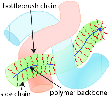
What does it take to design a polymer material that intrinsically avoids entanglement without using a large amount of solvent? William Daniel and his colleagues tackle this issue by designing a polymer chain geometry resembling a bottlebrush (shown in Figure 2). The bottlebrush geometry consists of a linear polymer backbone onto which short side chains, called bristles, are grafted. These bottlebrush-shaped chains are soft even in the absence of solvent. Instead of relying on small solvent molecules, bottlebrush networks use their bristles to keep polymer chains away from each other because bristles are too short to participate in the entanglement. As a result, the bottlebrush chains have an overall repulsion effect that resembles the repulsion effect of solvent molecules in hydrogels. Bristle repulsion allows bottlebrush polymers to surpass the elasticity of hydrogels! As an example, Figure 3 shows a compression test where a bottlebrush elastomer (on the right) retains its structure whereas a hydrogel material (on the left) fractures when compressed. Despite their similar elastic moduli, the bottlebrush elastomer displayed much greater compressibility than the hydrogel.
Figure 2. Schematic of three bottlebrush polymer chains. Each bottlebrush chain consists of a polymer backbone (linear chain) onto which short side chains (bristles) are attached. Figure adapted from the original article.
But what is an elastic modulus and why does it matter? The elastic modulus is a measure of the stiffness of a material and is given by the ratio of stress, the force causing deformation per area, to strain, the relative length by which the material is deformed by the stress. In these terms, a small modulus corresponds to low force per area resulting in significant deformation during compression – exactly what we expect of soft materials! As the entanglement density increases, a polymer chain network becomes more crowded resulting in a stiffer material [2]. Since bottlebrush bristles are too short to entangle, increasing the bristle density further reduces the entanglement density. Thus the elastic modulus of bottlebrush elastomers can be tuned by controlling the number of bristles grafted onto the polymer backbone. These bristles comprise the majority of the mass of the elastomer, e.g. 87% of the mass of the elastomer described in Figure 3.
Figure 3. Compression test of a hydrogel versus a bottlebrush elastomer. Left: PAM or poly(acrylamide) hydrogel made of 10% by weight polymer chains and 90% solvent. Right: bottlebrush elastomer made of 8% by weight backbone chains, 87% bristles and 5% solvent. Both materials have similar moduli (~2000 Pa). During compression, the bottlebrush elastomer kept its form while the hydrogel fractured. Figure adapted from the original article.
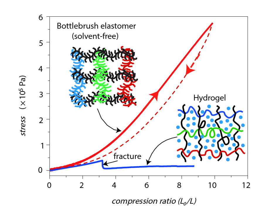
In addition to super-softness, bottlebrush networks are also highly compressible. The stress measurement in Figure 4 shows that bottlebrush elastomers (red curve) tolerated five times more stress before fracture compared to hydrogels (blue curve). Furthermore, the compression ratio (equilibrium length to compression length) of bottlebrushes was three times higher before fracturing. This means that bottlebrush elastomers are capable of sustaining much more deformation, and hence strain, than hydrogels.
Figure 4. Stress measured during compression of a bottlebrush elastomer (red curve) and a hydrogel (blue curve). The bottlebrush elastomer achieved a compression ratio (equilibrium length to compressed length) of about 10 while the hydrogel fractured at a compression ratio equal to 3. Image adapted from the original paper.
The idea of attaching bristles onto a polymer backbone in high density gave William Daniel and his colleagues control over the stiffness due to entanglement. This work expands scientists’ understanding of material properties consisting of branched polymer chains and points to a new frontier of dry supersoft materials. These new materials could play an important role in the development of soft robotics and synthetic biological tissues.
[2] In polymers, the entanglement contribution to the elastic modulus is given by the modulus equation:
Ge = neRT,
where ne is the number of chains involved in entanglement per unit volume, R is the universal gas constant, and T is the temperature. The modulus equation suggests that polymer materials become stiffer when heated. As temperature increases, the polymer network gains kinetic energy to attain structures with more “randomness”, or entropy. This increased randomness in polymer networks leads to more entangled states (higher entropy) that makes the material less prone to lengthening, hence more resistant to deformation.
Much of how DNA and proteins function depends on their conformations. Diseases like Alzheimers’ and Parkinsons’ have been linked to misfolding of proteins, and unwinding DNA’s double-helix structure is crucial to the DNA self-copying process. Yet, it’s difficult to study an individual molecule’s mechanical properties. Manipulating objects at such a small scale requires tools like optical and magnetic tweezers that produce forces and torques on the order of pico-Newtons, which are hard to measure accurately. One way around these difficulties is by modeling a complicated molecule as an elastic fiber that deforms in predictable ways due to extension and rotation. However, there are still many things we don’t know about how even a simple elastic fiber behaves when it is stretched and twisted at the same time. Recently, Nicholas Charles and researchers from Harvard published a study that used simulations of elastic fibers to probe their response to stretching and rotation applied simultaneously. The results shed light on how DNA, proteins, and other fibrous materials respond to forces and get their intricate shapes.
Before continuing, I would recommend finding a rubber band. A deep understanding of this work can be gained by playing along with this article.
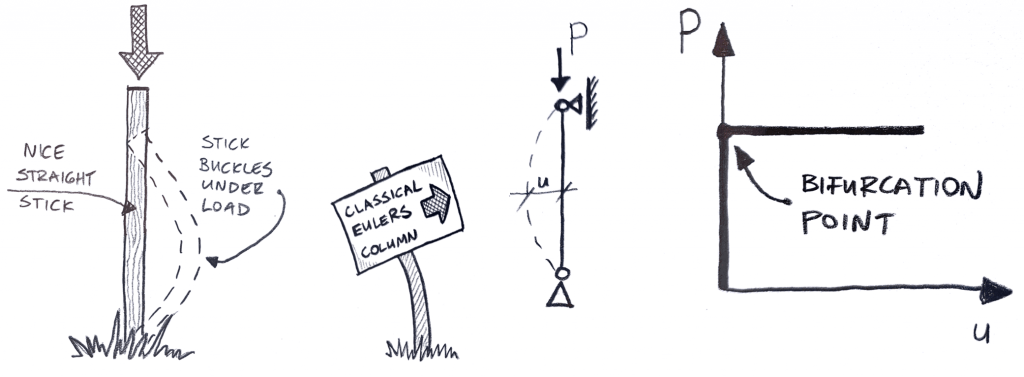
Long and thin elastic materials, (like DNA, protein, and rubber bands), are a lot like springs. You can stretch or compress them, storing energy in the material proportional to how much you change its length. However, compressing them too much may make the material bend sideways, or “buckle”. It might be more natural to think of this process with a stiff beam like in Figure 1, where a large compressive load can be applied before the beam buckles. But since your rubber band is soft and slender, it buckles almost immediately.
Figure 1. A straight, untwisted stick is compressed and buckles. It’s stiffer and thicker than your rubber band, so it sustains a higher load before buckling. (https://enterfea.com/what-is-buckling-analysis/)
Likewise, twisting your rubber band in either direction will store energy in the band proportional to how much it’s twisted. And, like compression, twisting can also cause it to deform suddenly. Instead of buckling, the result is a double-helix-like braid that grows perpendicular to the fiber’s length, as shown in Figure 2. An important caveat is that the ends of the rubber band are allowed to come together. But what happens when the ends of the band are fixed?
Figure 2. An elastic fiber is held with little to no tension and twisted. A double-helix, braid-like structure is formed. (Mattia Gazzola, https://www.youtube.com/watch?v=5WRkBWXUCNs)
Fixing the ends of a rubber band forces it to stretch as it twists. When this happens, a different kind of deformation can occur that combines extending, twisting, and bending the fiber. By stretching and bending simultaneously, the band forms a solenoid that is oriented along the long-axis of the band, reminiscent of the coil of a spring. An example of the solenoid shape appears in Figure 3.
Figure 3. An elastic fiber is held at high tension and twisted. A solenoid structure is formed. (Mattia Gazzola, https://www.youtube.com/watch?v=0LoIwE37aNo)
All of the phenomena described above can be seen by playing with rubber bands, yet a quantitative understanding of how these states form and how to transition between them has remained elusive. To tackle this problem, Charles and coworkers used a computer simulation to calculate the energy stored at each point along an elastic fiber when it is stretched and twisted. The simulated fiber was allowed to deform and search for its lowest energy configuration, a process critical to navigating the system’s instabilities and finding the state you would expect to find in nature.
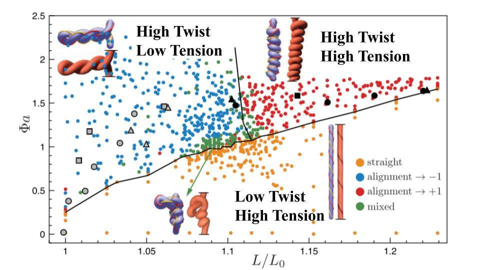
Figure 4 summarizes some of the different conformations attained by a fiber that is first stretched, then twisted to different degrees. We can see how a fiber with the same tension and different degrees of twist can lead to any one of a wide range of conformations. For instance, a fiber remains straight (yellow dots) when it’s stretched to a length $latex L$ that is 10% longer than its original length $latex L_{0}$ $latex (L/L_{0} = 1.1)$ until it is twisted by $latex \Phi a \approx 1$, where $latex \Phi a$ is the degree of twist multiplied by the fiber’s width divided by its length. Above this value of $latex \Phi a$, the simulated fiber twists into the braided helix structure seen in Figure 2 (blue dots). Likewise, when $latex L/L_{0} = 1.2$, the fiber remains straight until it has a much higher twist, $latex \Phi a \approx 1.5$, where it forms a solenoid (red dots).
Figure 4. Conformation of a simulated fiber under constant extension $latex L/L_{0}$, twisted by $latex \Phi$ normalized by the fiber dimensions $latex a$. Orange dots are straight, blue dots are double-helix braids, red dots are solenoids, and green dots are mixed states. Black and grey symbols are experimental results from a previous study.
Considering the vast understanding of the universe that physics has given us, it may be surprising that there is so much left to learn from the lowly rubber band. While it’s fun to play with, understanding the way fibers deform could help researchers understand all sorts of biological mysteries. For instance, your DNA is a unique code that contains all of the information needed to create any type of cell you have, but depending on where the cell is in your body, that same DNA only makes some specific cell types. The cell can do this by selectively replicating sections of its DNA while ignoring others. One way it does this is by hiding away certain regions of DNA through folding. Exploring the way simple elastic fibers deform could help explain the way DNA knows how to make the right cells, in the right places.
In my previous post on soft nanoparticles, you were introduced to polymer-based nanoparticles that could be used in biomedical applications, one of which is cancer therapy. These nanoparticles have a range of useful properties for cancer treatments, including their spherical shape and small size (~100 nm), both of which are similar to exosomes, small globules that are used in nature for transferring proteins between cells. Since cells naturally absorb exosomes, artificial particles with this size and shape should also be easy for cells to absorb, which means these particles could be used to deliver drugs into cells. While this idea sounds promising, it hasn’t worked out in practice — when drug-loaded polymer-based nanoparticles were injected into a tumor, subsequent tests showed that less than 1% of the injected dose entered the cancer cells. Since these particles were the correct size and shape, why didn’t they get inside the target cells?
One possibility is that the elasticity (or stiffness) of nanoparticles is to blame: scientists have suspected that this mechanical property can affect the ability of nanoparticles to squeeze themselves through the cell’s membrane. Unfortunately, it is difficult to test this hypothesis directly, because modifying the elastic properties of a nanoparticle generally requires modifying its chemical properties as well. To solve this problem, Peng Guo and coworkers designed a special kind of nano-objects — spherical nanolipogels — with tunable elasticity. In this paper, they proved for the first time that breast cancer cells take up soft, squishy particles more easily than they take up hard ones.
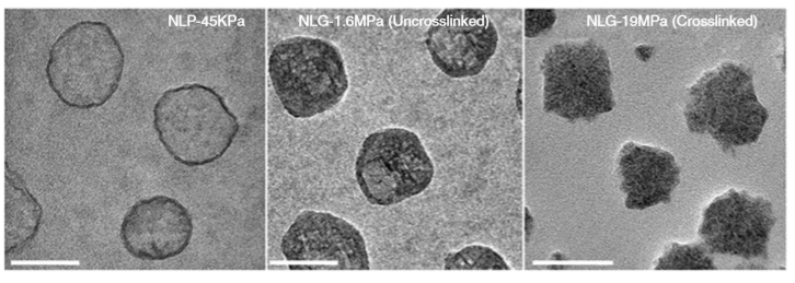
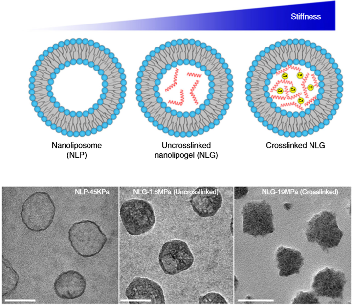
So what are nanolipogels? This type of nanoparticles is basically an altered version of a nanoliposome, a particle-like object that consists of a liquid water core surrounded by a layer of phospholipid molecules [1]. Guo and his colleagues created nanolipogels by filling the nanoliposomes’ liquid core with a polymer of tunable chemical structure. Nanolipogels have precise size (160 nm) and shape (spherical), and their elasticity can be made to vary without changing their other properties (see Figure 1).
Figure 1. Structures (top) and micrographs (bottom) of nanoliposomes and nanolipogels of increasing stiffness (higher values of Young’s modulus). (Image adapted from Guo’s paper.)
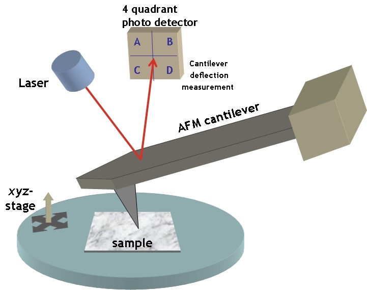
Figure 2. Experimental setup of an Atomic Force Microscope. The height of a sample’s surface is scanned by a tip on a moving cantilever and the cantilever deflections are detected by a laser light to give the samples topographic profile. (Image from simple.wikipedia.org)
To measure the elasticity of the particles they had produced, Guo and coworkers used a technique called Atomic Force Microscopy (AFM). AFM is commonly used to visualize soft materials by imaging the height of their surface through the deflection of a cantilever (Figure 2). In this paper, the researchers used AFM for a different purpose: to calculate the Young’s modulus — a measure of stiffness — of the nanoparticles. They did this by compressing the particles between the cantilever tip and a solid surface, allowing the researchers to measure the force required to deform the particles by some known amount. The relationship between the applied force, the degree of deformation, and the Young’s modulus is given by the Hertz equation [2]. What you need to remember is that the greater the modulus, the stiffer the particle.
The researchers created four different nanolipogels of different elasticity with Young’s moduli ranging from 1.6 MPa (roughly the stiffness of cork) to 19 MPa (the stiffness of leather), and a nanoliposome without polymer in the core with a Young’s modulus at 0.045 MPa (roughly the stiffness of gummy bears). After verifying that all 5 particles could successfully encapsulate drug molecules, they tested how well tumor cells could uptake each particle. To do so, they used breast cancer cells in the lab (in vitro cellular uptake) and attached fluorescent dye to the particles to determine whether they were inside or outside of the cells. They found that the stiffest nanolipogels were 80% less effective compared to the softest nanoliposome samples; in other words, five times more of the softer particles got inside the cells. In vivo tumor uptake studies, using live mice, similarly showed that the nanoliposomes had up to 2.6 times higher cellular uptake than the stiffest nanolipogels.
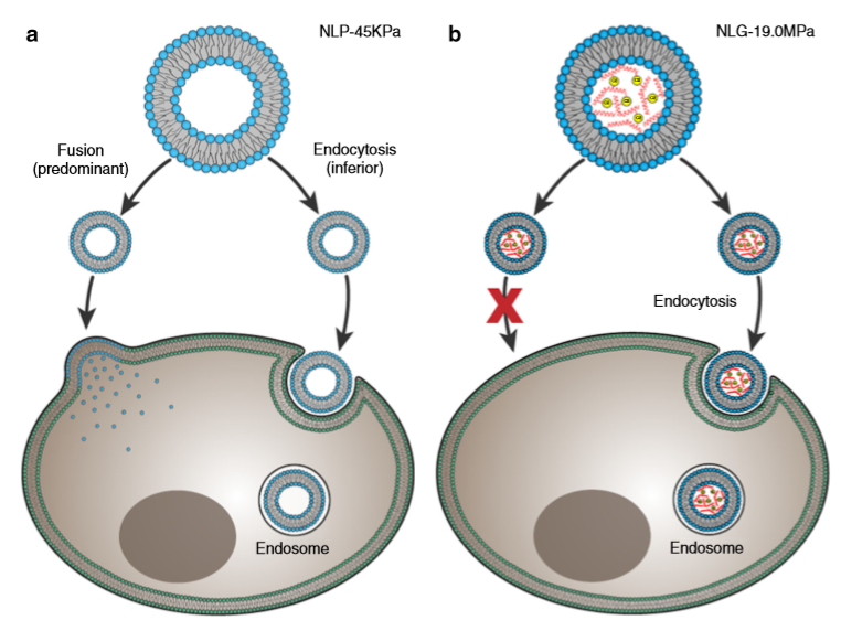
Why do the soft nanoliposomes enter the cells more easily? To understand the conclusion of Guo and colleagues, we need to think about how nano-objects enter a cell. Figure 3 shows two possible ways of doing this: 1. fusion, where nano-objects break up and join the cell membrane, or 2. endocytosis, where the whole object enters the cell by bending the cell’s membrane and getting covered in a membrane outer layer. Fusion needs less energy compared to endocytosis, where cell membrane bending and surface tension increase the energy. The researchers hypothesized that nanoliposomes use both fusion and endocytosis, with a preference for fusion (Figure 3a), while nanolipogels can only enter the cell through endocytosis (Figure 3b). This hypothesis was verified by using chemical compounds that prevented endocytosis from taking place; in all experiments, the cellular uptake of nanoliposomes was as high as before, while much fewer nanolipogels were detected in the cells, since they couldn’t enter through endocytosis.
Figure 3. The possible pathways of (a) nanoliposomes and (b) nanolipogels entering a cell. (Image adapted by the Guo paper.)
This study showed that a nanoparticle’s mechanical property, in particular, its elasticity, affects how it enters cells, a finding that could potentially have a tremendous impact on cancer treatment and diagnosis. The use of nanoliposomes, which are a synthetic equivalent of nature’s drug delivery systems, may also be used in the future to further understand how cellular processes, such as fusion and endocytosis, take place.
How an elastic beam deforms under load has been a question for as long as there have been engineers to ask it. In some cases, the force on a beam is approximated as a single point. For example, if a diving board is large enough, a diver at the end can be treated as a point mass on the beam. Another common approximation is to consider the force to be a continuous pressure along its length. Treating wind that bends a tree branch as a continuous pressure along the branch’s length is much simpler than adding up the force from every molecule of air on the branch. However, consider the case of a root growing into a granular material like soil. As the root burrows through the soil it will bend due to varying point-like forces along its length. The result is a branching and twisting root system that tries to grow along the path of least resistance. An example of the diversity in plant root morphologies is shown in Figure 1 and gives a sense of how complicated and interesting the physics behind this growth can be.
Figure 1. An example of the complex and diverse morphology of several types of plants which all live in the same ecosystem [1]
With this in mind, David J. Schunter Jr. et al. from the Holmes group at Boston University have developed a beautiful experiment to study what they call “elastogranular” phenomena. In their experiment, an elastic beam is inserted into a box which is filled at a particular density with uniform beads. An image of a typical experiment is shown in Figure 2. Once the beam reaches the end of the box it will not be able to penetrate any further, and trying to push more of the beam into the box will cause a compression along the beam’s length. This resembles a classic experiment where a beam is compressed in the same manner, but in the absence of beads. Compressing the beam against the end of the box becomes increasingly difficult until eventually the beam “pops” into one large buckle. In this simpler case, the beam was free to buckle with no restrictions. Introducing beads to the system reinforces the beam non-uniformly and constrains the shapes it can take on when it buckles. This complicates the buckling event and leads to interesting new behaviors.
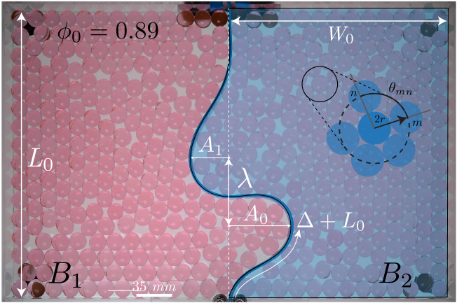
Figure 2. An elastic beam is inserted into a box of length $latex L_{0}$ and width $latex 2W_{0}$ filled with beads at an initial packing fraction of $latex \phi_{0} = 0.89$. After a length of beam is inserted equal to $latex L_{0}$, inserting additional length $latex \Delta$ results in buckling. In this experiment the beam takes on two buckles with wavelength $latex \lambda$, and amplitudes of $latex A_{0}$ and $latex A_{1}$ respectively.
In the experiment performed by the Holmes group, a beam is compressed against the end of the box until the beam buckles. If the packing fraction $latex \phi_{0}$ (the fraction of space within the box that is covered in beads) is low, it buckles much like one would expect in the absence of beads—one large buckle, as in Figure 3i. If $latex \phi_{0}$ is higher at the beginning of the experiment, like in Figures 3ii and 3iii, the buckling behavior becomes more complicated. The beam will form one large buckle as before, and as the buckle grows it will take up more area on one side of the box. This forces the beads to reorganize themselves, and the beads on the compressed side of the box become very tightly packed. At this point, they are in a hexagonal arrangement, and they are said to have crystallized [2]. As the beads in one side crystalize, that side becomes stiffer and suppresses further growth of the amplitude of the first buckle, $latex A_{0}$. In order to accommodate the extra length being inserted, $latex \Delta$, an additional buckle forms. The difference in buckling behavior for three values of $latex \phi_{0}$ are shown in Figure 3. [3]
Figure 3. Shape profiles of the inserted rod for various packing fractions ($latex \phi_{0}$) for the same normalized inserted length $latex \Delta/L_{0}$. i) At low $latex \phi_{0}$ the beam forms one large buckle. ii) As $latex \phi_{0}$ increases, the amplitude of the single buckle is suppressed, leading to a second buckle forming on the other side. iii) At even higher $latex \phi_{0}$, the buckles rotate and grow toward each other.
Figures 3 shows that not only are the number and amplitude of buckles significantly affected by the beads that surround the beam, but the orientations of the buckles are changed as well. When the experiment begins at a high $latex \phi_{0}$, the beam finds both sides of the box to be stiff and hard to penetrate. The initial buckle does not grow very much before the second buckle forms, and at high enough $latex \phi_{0}$ both buckles occur nearly simultaneously, forming a twin buckle. Figure 4 shows two systems with different $latex \phi_{0}$ forming twin buckles. In the top sequence where $latex \phi_{0}$ is lower, the buckles maintain a constant distance between each other as they grow since there are plenty of uncrystallized areas (light blue circles) ahead of the buckles into which they can grow. The lower sequence shows that, at higher $latex \phi_{0}$, the majority of uncrystallized beads are found in the wake of a buckle so the buckles instead grow into these regions, as demonstrated by the red lines.
Figure 5. Twin buckles increase in amplitude as $latex \Delta$ increases (left to right) growing into less-dense, uncrystallized regions (light blue circles). For lower $latex \phi_{0}$ (top sequence), uncrystallized beads in front of the buckles can be pushed aside, crystallizing beads away from the buckles (dark blue and yellow circles). At higher $latex \phi_{0}$ (lower sequence), the uncrystallized sections occur behind the buckles, causing the two buckles to grow closer together which is shown by the red lines.
This system bears a striking resemblance to that of plant roots growing into the soil and could be useful in understanding how environmental pressures cause plant root systems to evolve. For example, cacti need to absorb as much water as they can from their environment. One way of accomplishing this is to increase the surface area of the root system by growing wide and close to the surface, rather than deep, in order to collect water from a larger area. By developing thin roots that buckle before they can deeply penetrate the soil, many cacti are able to produce the shallow, wide-reaching roots system they need to find water.
David J. Schunter Jr. and coworkers have shown that combining two well-understood problems—buckling of a beam and reorganization of beads—can lead to unique and interesting bending dynamics. By confining a beam to a box of beads, the buckling of the beam becomes strongly influenced by the packing fraction and reorientation of the beads. This particular system shows a strong resemblance to plant root growth, but also be informative for synthetic applications involving the insertion of flexible filaments into deformable materials.
[2] When spheres crystallize in two dimensions, the hexagonal lattice is the closest possible packing with an area fraction of $latex \phi = 0.9069$. Interestingly, Figure 3iii shows a packing fraction of 0.91, which is higher than this maximum value. This is because the beads are able to pop out of the plane at very high compressions, which can lead to a calculated packing fraction larger than that of the hexagonal lattice. For more information on hexagonal packing, see Wikipedia.
[3] For more information about the specifics of how the deformation of the beam is quantified, a summary of the analysis is available here.
I’m going to start this post with an experiment. Find a piece of smooth and unwrinkled A4 or paper of a similar size, and hold it by gripping an edge between your thumb and forefinger. Due to the gravitational force, the paper is pulled down and is bent. Now crumple the same paper, then unfold and hold it by the edge again. What happened? The paper can now resist gravity! This wrinkling strategy is a simple trick to improve the mechanical response of a thin 2D sheet. Astonishingly in biology, by such simple ways, cells tune the mechanics of their thin membrane to form tiny capsules called vesicles in order to uptake nutrients, to dump waste, and to communicate. But how such a thin sheet can address all these needs? What are the mechanisms behind these tunings? Are there consequences other than mechanical improvements? In today’s paper, Changjin Huang and colleagues investigate the critical parameters governing the vesicle formation process (or vesiculation) and the size distribution of vesicles.
The Vesiculation Process
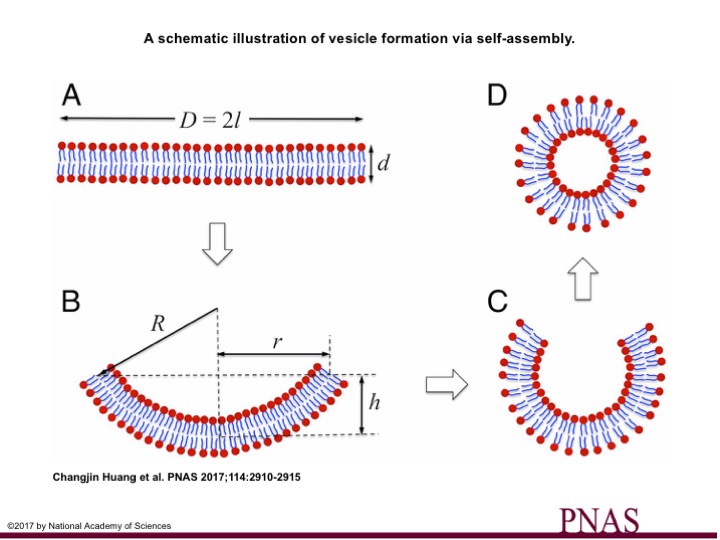
A class of molecules called amphiphiles contain two parts: a water-loving (hydrophilic) head and a water-fearing (hydrophobic) tail. When amphiphiles are dispersed in water, the hydrophobic tails are frustrated and get together (self-assemble) to stay away from water. Based on the geometry of these two parts, different structures emerge (see note [1]). One such structure is the bilayer structure (Fig. 1A).
Fig. 1. A through D is the evolution of a vesicle, starting from a membrane patch (A) bending to (B) and closing at (C ) to form vesicles. The spontaneous decrease in systems’ energy by closing the patch is opposed by the energy required to bend the patch. The competition between these two energies is determined by factors such as patch size(l), membrane thickness (d), curvature (1/R), and bending stiffness ($latex k_b$). Combination of any of these factors can result in either or combination of above morphologies.
A bilayer structure composed of two layers of molecules with the hydrophobic tails turned inward (Fig 1A). This bilayer arrangement still is not the favored structure, since the water-fearing tails are exposed to water on the edges of the bilayer. An energy is imposed on the system by such exposure. This energy is called the interface energy and usually is shown by ?. This interfacial energy is the only driving force for the bilayer to bend in order to minimize the system’s energy. Thereby, the bilayer attempts to bend into spherical structures (Fig 1B & C). But bending comes at a cost! The system needs to exert force to bend the bilayer. In other words, energy is required to curve the bilayer. In this work, Huang and colleagues model this process with an energy-minimization approach to realize the critical parameters that determine the fate of this competition.
Parameters Affecting the Vesiculation
The quick paper experiment highlighted the essential role of local curvature in sheet’s rigidity, but that’s not all. The authors of this study theoretically demonstrate that besides local curvature, membrane thickness, membrane bending resistance (bending stiffness) and the membrane patch size (size of the paper sheet) all play a crucial role in the vesiculation process. When the authors considered the role of membrane thickness, they could predict morphologies other than vesicles such as disks and cups which we observe in real-life experiments.
Many models have been developed in recent decades to explain the vesiculation process, and none were able to predict the intermediate morphologies. In all of these models, the membrane is treated as a 2D sheet with no thickness such that when it is bent, only undergoes linear elastic deformation. Before we proceed, let’s briefly elaborate on ” linear elasticity”.
Imagine a spring that is being pulled by a force that you apply. The magnitude of extension is proportional to the force exerted. This example corresponds to a linear response. However, there is a threshold force after which the extension magnitude is not proportional to the force, and to predict the behavior of spring, you may need to consider non-linear terms in the model. The same consideration applies to the vesiculation process. To model the energy required to bend a membrane patch we need to consider non-linear terms since our material is a very, very thin 2D sheet undergoing an enormous deformation when bent. So, for small bendings, the small value of $latex h$ in Fig 1B, the linear term will suffice. But if membrane bends to final stages of closing itself, larger $latex h$, then we need to consider the non-linear term as well.
With this combination of linear and non-linear terms, an energy minimization model is proposed by the authors upon which a critical membrane bending length is obtained. At lengths, smaller than the critical length, the bending energy barrier increases dramatically, making it hard for the membrane to bend. At lengths larger than the critical length, bending energy barrier tends to zero and the membrane can readily bend (see note [2]). Now if we know the parameters to change this critical length, then we would be able to alter the vesicle size or to understand the mechanics of different vesicles produced by both healthy and diseased cells.
Effect of Curvature
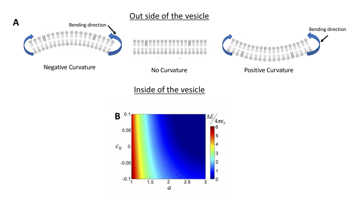
The proposed model in the original study reveals that by introducing wrinkles, we can modify the critical length, however, the model also shows that decrease or increase of the critical length by wrinkles (or membrane spontaneous curvature-see note [3]) depends on curvature direction. Under negative spontaneous curvature, the membrane is curved in the opposite direction of bending (Fig 2A). Under this condition, the model shows that the critical length is larger than when the spontaneous curvature is positive. Note how in Fig 2B, for a negative curvature the bending energy barrier diminishes only at larger critical length. So, if a given membrane bilayer has specific molecules mostly inducing negative curvature, the critical length for that membrane will be larger, meaning that the patch needs to grow more to reach the critical length after which there would be no barrier for bending. Under such condition, larger vesicles will form in contrast to the membrane with positive spontaneous curvature, which can bend itself at lower critical length, thus, forming small vesicles.
Fig 2. Effect of spontaneous curvature on membrane critical length. (A) schematics showing two types of curvatures; positive (left) and negative (right) both under same bending direction. (B) Total bending energy is calculated with respect to the spontaneous curvature, $latex c_0$ and the critical length, $latex a$. The heat map shows the barrier energy for bending. Amphiphilic molecules shown with darker tails were aimed to induce curvature based on their geometries.
Effect of Membrane Bending Stiffness
Bending stiffness, shown by $latex k_b$ is the bending resistance of the membrane and thus it is a membrane property. Sometimes cells recruit molecules such as cholesterol to their membrane to increase the membrane bending stiffness. On the other hand, viruses are known to decrease the membrane stiffness so that they can readily bend the host’s cell membrane. In regard to vesicle size distribution analysis, the proposed model showed that the critical length is proportional to bending stiffness. In other words, for the stiffer membrane, the critical length is larger and these membranes tend to form larger vesicles.
Effect of Membrane Thickness
So far, for our analysis of the membrane (or sheet for our analogy) thickness was fixed. To consider the membrane thickness, the authors adopt a simple approximation. They first argue that membrane stiffness varies as a function of membrane thickness squared ($latex k_b \propto d^2$). Then, assuming that membrane is free to bend (its size is larger than the critical length), they obtain the minimum diameter of the vesicle formed from this membrane size as $latex D_{min}=(critical\ length) + (membrane\ thickness)$. But $latex critical\ length \propto k_b$. Therefore, from their argument we can write:
$latex D_{min}=d^{2} + d$
With this approach, membrane thickness is considered as a non-linear concept. The proposed model reveals that for thicker membrane the critical length is larger, and thus these membranes will more likely form larger vesicles. In contrast, for the thinner membranes, the critical length is shorter and these membranes are prone to form small-sized vesicles.
Conclusion
The vesiculation model developed by Huang and his colleagues has contributed to our understanding of how vesicles form. Understanding the parameters that govern vesicle formation is critical for the design of vesicles for applications such as drug delivery, where nanoscale vesicles are needed to move drugs into a cell. In addition, the identified vesiculation parameters could be used as diagnostic measures, as it has been shown that the vesicles produced by cancer cells or by cells infected with viruses have mechanical properties different from healthy cells.
[1] Known as Israelachvili’s packing parameter, the volume of the hydrophobic part divided by the product of effective hydrophilic area and the length of the hydrophobic part,$latex p=\dfrac{v}{l*a}$, defines the favored morphology. when p < $latex \frac{1}{3}$ spherical micelles, $latex \frac{1}{3}$ < p < $latex \frac{1}{2}$ cylindrical micelles, p > $latex \frac{1}{2}$ bilayer structures are expected to form.
[2] Cut an unwrinkled A4 paper in half and see the bending response. If you continue cutting you will notice that after a certain length the paper doesn’t bend. That length is the critical length.
[3] Spontaneous curvature is the natural curvature of the membrane because of asymmetries between two monolayers of the bilayer. These asymmetries can be due to the presence of proteins or geometrical difference of different amphiphilic molecules making the membrane.