Standing in the center of a crowded bus on your way to class, you might think: “why don’t these people just move? It’s hot and I can’t breathe!” Male penguins huddling to keep their eggs warm in the Antarctic winter have the opposite problem – no penguin wants to be at the cold edge of the huddle. A penguin in the huddle wants to stay in the warm center, since the outside temperature can reach -45 oC. However, penguins on the edge of the huddle are trying to push through the crowd to reach the center. Through the independent motion of each penguin, the huddle stays tight enough for the center to remain warm but loose enough to keep moving.
In today’s study, Zitterbart and colleagues investigate how huddling Emperor penguins can keep moving, as in this video. They find that individuals take small, coordinated steps that reorganize the huddle on a time scale of hours.
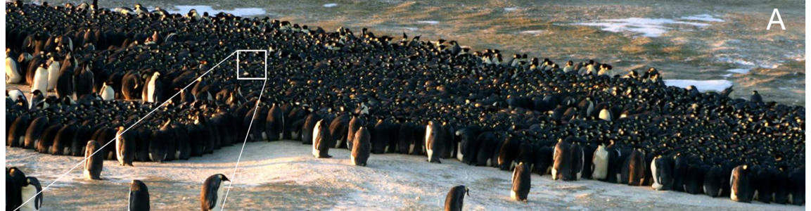
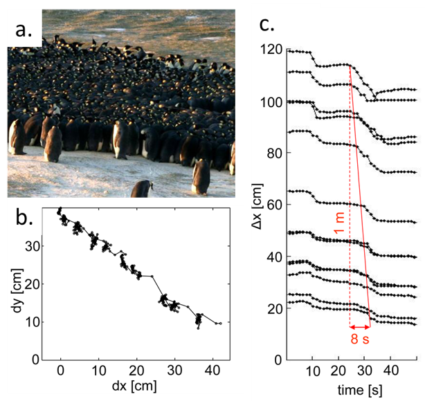
Zitterbard and colleagues film a 2000-penguin colony (shown in Figure 1a) for 4 hours and track the positions of the penguins, with an x-coordinate corresponding to horizontal position on the camera image and y-coordinate corresponding to the vertical position on the camera image. When huddling, the penguins all face in the same direction and are arranged roughly in a hexagonal grid. Every 30 to 60 seconds, the penguins take small steps, 5-10 cm long. Figure 1b shows the track of one penguin, with a point every 1.3 seconds. There are clusters of points where the penguin is standing still (with no significant change in position), and then a straight line when the penguin takes a step.
Since penguins at one spot in the huddle don’t know that another part of the huddle is moving, they don’t all step at once. Instead, there is a wave of moving penguins that moves through the huddle at a speed of 12 cm/s, like a sound wave traveling through a material. Figure 1c shows the tracks of several penguins at the same y-position and different x-positions in the huddle. Their horizontal motion is correlated – the penguin at the top track moves first, and then the motion propagates to the neighboring penguins as a wave.
Figure 1. a. A photograph of huddling penguins with x- and y- coordinate axes. b. A track of a single penguin with points every 1.3 seconds. Clusters of points mean the penguin isn’t moving, and a straight line means the penguin took a step. c. Horizontal motion of several penguins. These penguins are at the same vertical position in the huddle but different horizontal positions. The slope represents the 12 cm/s motion of the wave of moving penguins.
An unusual aspect of this study is that the results section is short – the authors only report the traveling wave of penguins through the huddle. However, they then move to an explanation of penguin motion using very interesting analogies to granular materials (such as sand or coffee beans).
There are three effects of the small steps:
They allow the penguins to reach the best density for warmth.
They move the entire huddle forward, and merge small huddles into big ones.
They reorganize the huddle, allowing penguins to leave the huddle at the front and join it at the back.
The combination of small penguin movements and organized huddling is similar to the way colloids [1] solidify when the particles in the colloid attract one another. Penguins huddle when they are “attracted” to each other by cold temperatures; colloids are attracted by electrostatic or intermolecular van der Waals forces. Thinking of a group of organisms as a fluid, such as smoothly flowing fish schools and turbulent bacteria, is a well known method for understanding their behavior. In contrast, the small steps in a dense group of penguins is reminiscent of a material going from a fluid to a solid state. The waves in the huddle are similar to waves in other groups of animals, like human crowds rushing to escape a room. Luckily, the penguin waves do not result in injury. (Usually.)
Through small, careful steps, penguins are able to create a solid cluster of warmth in the Antarctic winter. If we took a hint from the penguins and were more careful about our motion when on a crowded subway, maybe our commutes would be much more pleasant experiences. Of course, the huddling penguins are not bounded by the walls of a bus – how they would move if they didn’t have an open boundary is still a mystery!
[1] Mixtures of small particles dispersed throughout another substance, such as the fat suspended in a water solution to form milk.
We are surrounded by phenomena caused by the scattering of light. When enjoying a sunny day at the seaside, like in the photo at the top, why is the sky blue? Blue light scatters more than red light. Why is milk opaque? Protein and fat particles scatter light. If you are reading this with blue eyes, your eye color is due to light scattering. Scientists use the same general scattering principle to study the structure of soft materials using the scattering of well-defined radiation. Scattering measurements reveal structures between an ångström and hundreds of nanometers, an important region for studying soft matter. Just as the color of the sky results from light scattered by air molecules, the scattering of X-rays and neutrons tells us about the size and shape of compounds in soft materials along with their interactions, and I will focus on these two types of radiation.
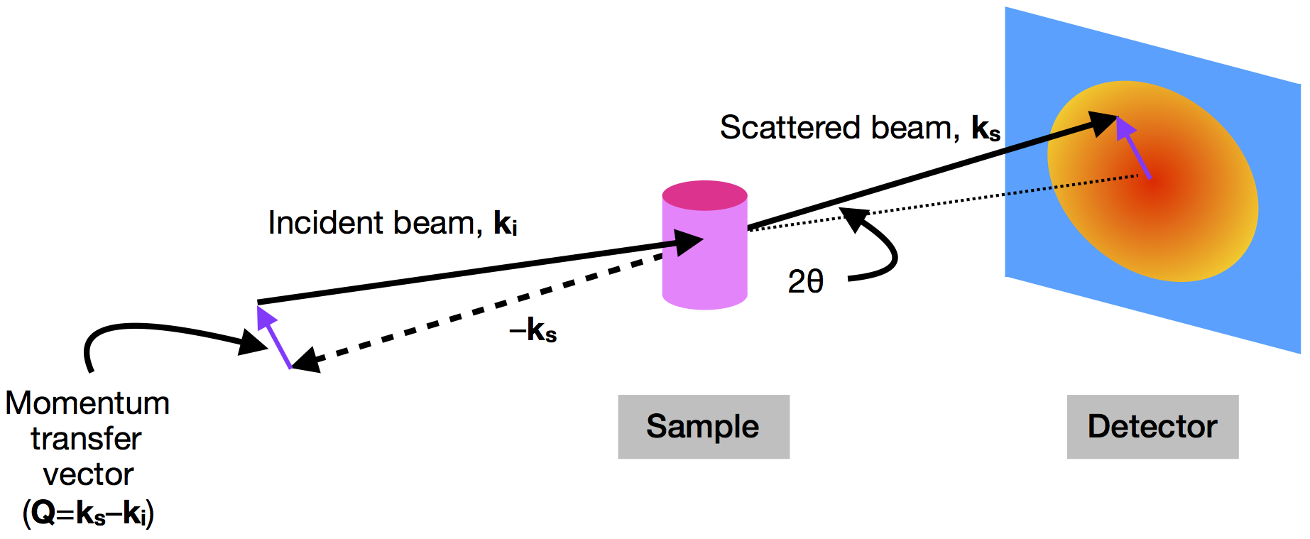
In a small-angle scattering experiment (SAXS when using X-rays and SANS when using neutrons), a sample (whether solution, dispersion, or solid) is placed between an incoming beam of radiation and a detector (see Figure 1) [1]. The detector measures the scattering intensity as a function of angle, which in turn can be related to the size and shape of the sample’s components.
Scattering intensity is quantified as a function of the momentum transfer vector (or scattering vector) $latex \mathbf{Q}$, which is simply the difference between the momentum of the incoming beam ($latex \mathbf{k_i}$) and the scattered beam ($latex \mathbf{k_s}$). The magnitude of $latex \mathbf{Q}$ (equal to $latex (4 \pi \sin{\theta}) / \lambda$) depends on the scattering angle ($latex 2 \theta$) and the wavelength of the radiation ($latex \lambda$) [2].
Figure 1. The geometry of a small-angle scattering instrument. An incident beam of X-rays or neutrons (with momentum $latex \mathbf{k_i}$) is scattered by a sample with an angle of $latex 2 \theta$. The scattered beam (with momentum $latex \mathbf{k_s}$) is then detected at a point beyond the sample. The difference in momentum between the incident and scattered beams is $latex \mathbf{Q}$. (Image produced by the author.)
The relationship between the magnitude of $latex \mathbf{Q}$ and the length scale being investigated ($latex d$) is given by the equation $latex Q = 2 \pi / d$, and this inverse relationship to distance is why measurements as a function of $latex Q$ are said to be in reciprocal space. (This relationship comes from Bragg’s law for crystals [3].) In real space, the arrangement of objects is described by the distances between them. In reciprocal space, the same arrangement would be given by $latex Q$. The scattering process is essentially a Fourier transform [4], a mathematical procedure to convert waves to frequencies, making it possible to go between real and reciprocal spaces.
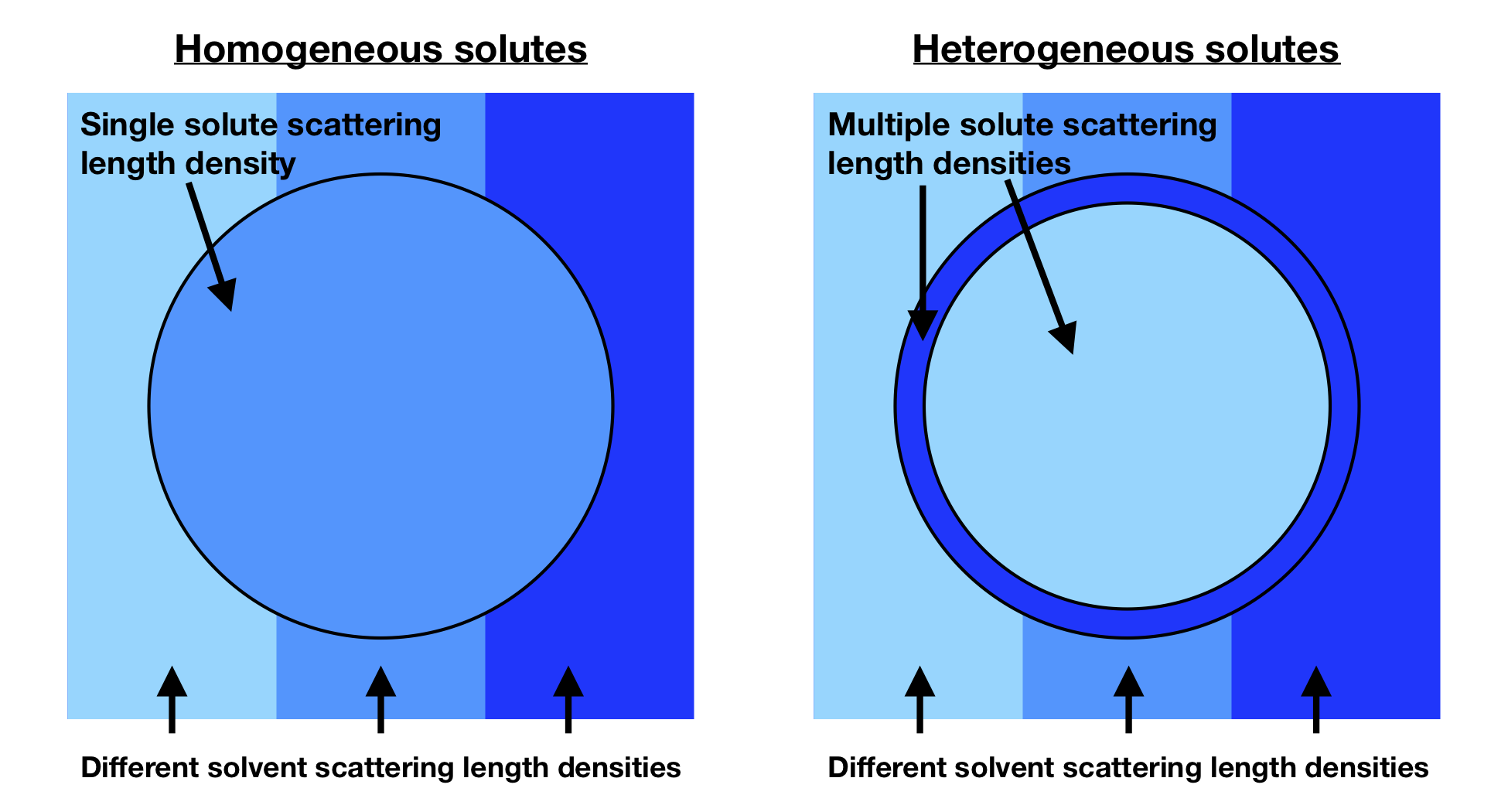
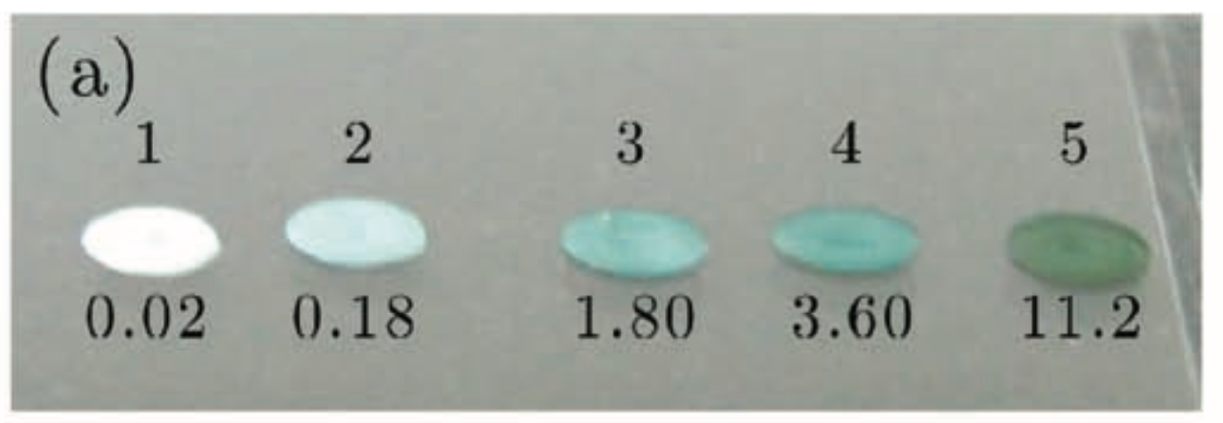
Now, having established some of the fundamentals of waves and scattering, we need to think about how radiation interacts with materials. This interaction determines the way that scattering data look and also what information you can obtain. Specifically, X-rays interact with electrons, and neutrons interact with nuclei. The magnitude of the interaction is quantified by the amount per volume (the “scattering length density”), and a difference in scattering length density between solutes and solvents results in detectable scattering. The scattering length density can be thought of as the “refractive index” for neutrons or X-rays. Figure 2 shows the general idea of contrast for any scattering experiment, with a comparison between homogeneous and heterogeneous solutes. When the color of the solvent and particle are the same shade of blue (meaning they have the same scattering length density), there is no scattering from that component. When the colors are different (meaning that they have different scattering length densities), there is now scattering.
Figure 2. Schematic of how the contrast between solutes (circle) and solvents (surrounding) for solvents and solutes with different scattering length densities gives rise to scattering. When the two colors are matched, which is possible for homogeneous solutes (left), there is no scattering. For heterogeneous solutes (right), there is no one solvent that can match the entire particle. (Image produced by the author.)
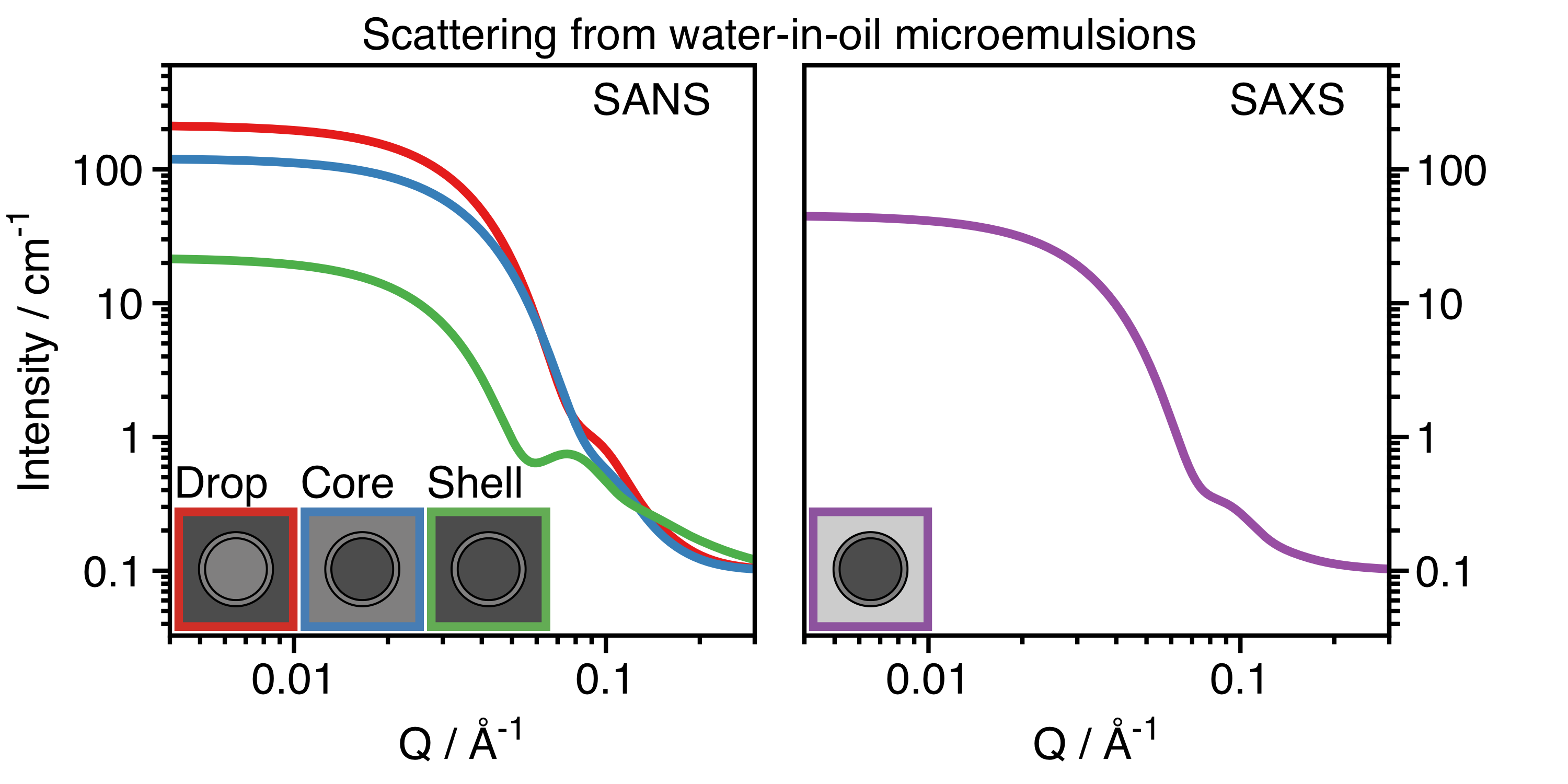
Interactions between X-rays and materials are fixed by their composition. However, neutrons interact differently with different isotopes of the same element. One particularly useful difference, especially for soft organic materials, is for structures with protons (1H) and those where protons are exchanged for deuterons (2H or D) [5]. It is possible to detect scattering from specific parts of complex systems by tuning the contrast of different components using solvents with different contrasts, as shown in Figure 2. Figure 3 shows calculated SANS (left) and SAXS (right) curves from chemically identical but isotopically distinct microemulsions, which are nanometer-sized droplets of water that are surrounded by surfactants in oil [6]. For the SANS curves, the dark grey areas represent deuterated oil or water (called D2O or heavy water), and the light grey areas represent standard hydrogenous oil or water. Multiple contrasts are required for a heterogenous particle, because no single solvent can match the whole particle (Figure 2, right). The curves are all different, but the actual structure of the microemulsion is always the same. It is only the contrast that differs. A precise determination of the structural dimensions of the microemulsion can be determined by analyzing all the data together, which gives more certainty than considering any one alone.
Figure 3. Scattering intensity as a function of the $latex Q$ for water-in-oil microemulsions calculated for SANS (left) and SAXS (right). For the three SANS curves measured, the dark grey regions are deuterated water (D2O) or deuterated oil, and the light grey regions are standard water (H2O) or oil. For drop contrast (red), you detect surfactant and water. For core contrast (blue), you detect water only. For shell contrast (green), you detect surfactant only. For the SAXS curve (purple), the contrast is fixed, and the water core dominates. (Image produced by the author.)
Scattering data is analyzed by comparing experimental data to known equations for how different shapes should scatter radiation as a function of $latex Q$. Luckily, many models are already known [7] for various shapes. However, as structures are determined somewhat indirectly from the scattering data, complementary information from other techniques, such as microscopy, is frequently obtained as well. The equation relating the shape and scattering as a function of $latex Q$ is called the “form factor”, an intraparticle property. For example, the curves in Figure 3 were all calculated using a form factor for a particle consisting of a spherical core surrounded by a shell of another material. At the extremes of $latex Q$, approximations can be used to calculate the size (at low-$latex Q$) and the interfacial roughness (at high-$latex Q$). In addition, the size distribution usually must be considered. In the example in Figure 3, the radii of the cores do not have a single value. There is a size distribution of about 20%.
For more concentrated dispersions or for more strongly interacting systems, the interactions between the particles must be considered. In these cases, an interparticle property called the “structure factor” contributes to the shape of the scattering curves. It can be calculated for particles that are considered to interact as hard spheres, charged spheres, or attractive spheres. Often samples are studied dilute to avoid the structure factor contribution. However, for systems that are necessarily concentrated or charged, it must be accounted for.
In this post, I focussed on the fundamentals of scattering with examples from nanoparticle dispersions in dilute conditions. However, these are not the only kind of soft materials that can be studied. Polymer solutions and blends, complex fluids, liquid crystals, gels, and a variety of biological materials (such as proteins and nucleic acids in solution or lipid bilayers) can be studied using small-angle scattering. The properties of soft materials often emerge out of their structures. By characterizing them in a quantitative way, scientists can determine the relationships between structures and their functions. Using small-angle scattering, we can not only better understand materials but also better predict ways of improving them. Small-angle scattering should be one of the tools employed by everyone interested in soft materials.
The featured image at the top is a photo of Bellevue Beach in Klampenborg in Copenhagen, Denmark. (Image taken by the author.)
[2] The angles being scattered are truly small, typically on order of 1° or less. By using $latex Q$, it is both the wavelength and angle that are important, and conveniently measurements performed using different wavelengths can be directly compared. ^
[3] Bragg’s law gives the conditions that a wave is diffracted by a series of planes. In a crystal diffraction measurement, peaks are observed in the data when Bragg’s law conditions are met. In a scattering measurement, where Bragg peaks are seldom observed, the relationship between $latex Q$ and $latex d$ is useful as a ruler for the length scale that is being examined. ^
[4] A Fourier transform is a mathematical operation that turns a periodic function, like a wave, into a probability of different frequencies. If, for example, you had a wave with a single wavelength, its Fourier transform would give a 100% probability at that wavelength. ^
[5] Deuterium is the heavy isotope of hydrogen with one neutron and one proton. ^
[6] A microemulsion is not just a small emulsion. Although, both are dispersions of two immiscible liquids, typically stabilized by a surfactant. A microemulsion is thermodynamically-stable and, in the case of a water-in-oil rather than oil-in-water, can be thought of as water-swollen surfactant micelle. Data for Aerosol OT-stabilized water-in-oil microemulsions can be found in the PhD thesis “Phase behaviour and interfacial properties of double-chain anionic surfactants” by Sandine Nave (University of Bristol). ^
There are many things that we “know” about the world around us. We know that the Earth revolves around the Sun, that gravity makes things fall downward, and that the apparently empty space around us is actually filled with the air that we breathe. We take for granted that these things are true. But how often do we consider whether we have seen evidence that supports these truths instead of trusting our sources of scientific knowledge?
Students in school are taught from an early age that matter is made of atoms and molecules. However, it wasn’t so long ago that this was a controversial belief. In the early 20th century, many scientists thought that atoms and molecules were just fictitious objects. It was only through the theoretical work of Einstein [1] and its experimental confirmation by Perrin [2] in the first decade of the 20th century that the question of the existence of atoms and molecules was put to rest. Today’s paper by Newburgh, Peidle, and Rueckner at Harvard University revisits these momentous developments with a holistic viewpoint that only hindsight can provide. In addition to re-examining Einstein’s theoretical analysis, the researchers also repeat Perrin’s experiments and demonstrate what an impressive feat his measurement was at that time.
In the mid-1800s, the botanist Robert Brown observed that small particles suspended in a liquid bounce around despite being inanimate objects. In an effort to explain this motion, Einstein started his 1905 paper on the motion of particles in a liquid with the assumption that liquids are, in fact, made of molecules. According to his theory, the molecules would move around at a speed determined by the temperature of the liquid: the warmer the liquid, the faster the molecules would move. And if a larger particle were suspended in the liquid, it would be bounced around by the molecules in the liquid.
Einstein knew that a particle moving through a liquid should feel the drag. Anyone who has been in a swimming pool has probably felt this; it is much harder to move through water than through air. The drag should increase with the viscosity, or thickness, of the fluid. Again, this makes sense: it is harder to move something through honey than through water. It is also harder to move a large object through a liquid than a small object, so the drag should increase with the size of the particle.
Assuming that Brownian motion was caused by collisions with molecules, and balancing it with the drag force, Einstein determined an expression for the mean square displacement of a particle suspended in a liquid. This relationship indicates how far a particle moves, on average, from its starting point in a given amount of time. He concluded that it should be given by
where R is the gas constant, T is the temperature, $latex \eta$ is the viscosity of the liquid, $latex N_A$ is Avogadro’s number [3], r is the radius of the suspended particle, and $latex \tau$ is the time between measurements [4]. With this result, Einstein did not claim to have proven that the molecular theory was correct. Instead, he concluded that if someone could experimentally confirm this relationship, it would be a strong argument in favor of the atomistic viewpoint.
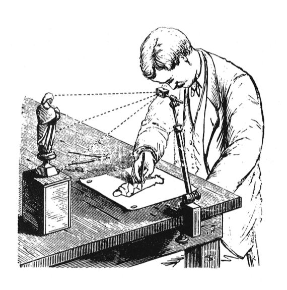
Figure 1: A camera lucida is an optical device allows an observer to simultaneously see an image and drawing surface and is therefore used as a drawing aid. (Source: an illustration from the Scientific American Supplement, January 11, 1879)
This is where Perrin came in. Nearly five years after Einstein’s paper was published, he successfully measured Avogadro’s number using Einstein’s equation, confirming both the relationship and the molecular theory behind it. However, with the resources available at the time, this experiment was a challenge. Perrin had to first learn how to make micron-size spherical particles that were small enough that their Brownian motion could be observed, but still large enough to see in a microscope. In order to measure the particles’ motion, he used a camera lucida attached to a microscope to see the moving particles on a surface where he could trace their outlines and measure their displacements by hand. Perrin obtained a value of $latex N_A = 7.15 \times 10^{23}$ by measuring the displacements of around 200 distinct particles in this way.
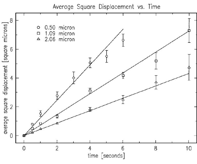
Performing this experiment in the 21st century was much simpler than it was for Perrin. Newburgh, Peidle, and Rueckner were able to purchase polystyrene microspheres of various sizes, eliminating the need to synthesize them. They also used a digital camera to record the particle positions over time instead of tracking the particles by hand. Using particles with radii of 0.50, 1.09, and 2.06 microns, they measured values of $latex 8.2 \times 10^{23}$, $latex 6.4 \times 10^{23}$, and $latex 5.7 \times 10^{23}$. Perhaps surprisingly, even with all of their modern advantages, the researchers’ results are not significantly closer to the actual value of $latex N_A = 6.02 \times 10^{23}$ than Perrin’s was a hundred years earlier.
Figure 2: Einstein’s relationship predicts that the mean square displacement should be linear in time. By observing this relationship for three different particle sizes, the researchers use the slope to obtain three measurements of Avogadro’s number. (Newburgh et al., 2006)
For those of us who work in the field of soft matter, the existence of Brownian motion and the linear mean square displacement of a particle undergoing such motion are well-known scientific facts. The authors of this paper remind us that, not so long ago, even the existence of molecules was not generally accepted. And, although we often take for granted that these results are correct, first-hand observations can be useful for developing a deeper understanding and appreciation: “…one never ceases to experience surprise at this result, which seems, as it were, to come out of nowhere: prepare a set of small spheres which are nevertheless huge compared with simple molecules, use a stopwatch and a microscope, and find Avogadro’s number.” [5]
[1] A. Einstein, “On a new determination of molecular dimensions,” doctoral dissertation, University of Zürich, 1905.
[2] J. Perrin, “Brownian movement and molecular reality,” translated by F. Soddy Taylor and Francis, London, 1910. The original paper, “Le Mouvement Brownien et la Réalité Moleculaire” appeared in the Ann. Chimi. Phys. 18 8me Serie, 5–114 1909.
[3] Avogadro’s number is the number of atoms or molecules in one mole of a substance.
[4] In 1908, three years after Einstein’s paper, Langevin also obtained the same result using a Newtonian approach. (P. Langevin, “Sur la Theorie du Mouvement Brownien,” C. R. Acad. Sci. Paris 146, 530–533 1908.)
[5] A. Pais, Subtle Is the Lord (Oxford U. P., New York, 1982), pp. 88–92.
What is the first thing that comes to mind when you hear the word mucus? For most people, it’s probably the last time they had a cold. Mucus is not usually something we think about unless there’s a problem. However, it is always there, working behind the scenes to make sure that our bodies function smoothly. Mucus lines the digestive, respiratory, and reproductive systems, covering a surface area of about 400 square meters- about 200 times more area than is covered by skin. In addition to providing lubrication and keeping the underlying tissue hydrated, mucus also plays a key role the human immune system. It serves as a selectively permeable membrane that protects against unwanted pathogens while also helping to support and control the body’s microbiome [1].
Mucus is an example of a hydrogel, which is a three-dimensional polymer network that is able to hold a large amount of water. While hydrogels get their structural integrity from this polymer network, the polymer makes up only a small fraction of the material once they are swollen with water [2]. In mucus, this network is made of biopolymer called mucin.
Researchers in the Ribbeck lab at MIT think that mucus is an underappreciated–and understudied–part of the human body. They have developed techniques for characterizing the mucus hydrogel to better understand how it is able to function as a selective filter. In today’s paper, Kathryn Smith-Dupont and coworkers in the Ribbeck lab investigate cervical mucus and try to understand the relationship between mucus permeability, or its ability to be a selective filter, and the risk of preterm birth.
A birth that occurs before 37 weeks of gestation is considered a preterm birth. This can be associated with negative health outcomes for the baby both in infancy and later in life. Preterm birth is the leading cause of death for children 5 years of age and under, and those who survive can face challenges such as learning disabilities and hearing problems [3]. While the causes of preterm birth can be complex and varied, infection in the fluid surrounding the fetus–which is known to trigger preterm birth–is seen in 25-40% of cases. The infecting bacteria are often the same species that are found in the vagina, suggesting that it traveled through the cervical mucus barrier to infect the sterile uterus.
Smith-Dupont and coworkers look for correlations between mucus permeability and preterm birth risk by comparing the cervical mucus in ovulating non-pregnant women with that in pregnant women. Once the pregnant women give birth, their mucus is characterized as low-risk or high-risk depending on whether they had a preterm birth. The cervical mucus in ovulating non-pregnant women is expected to be at its most permeable to facilitate the passage of sperm, whereas in pregnant women the mucus should be less permeable. Whether a microbe makes it through the mucus barrier can be affected by its size, biochemical interaction with the mucin, or a combination of the two.
First, the researchers look at the permeability of the mucus to 1-micrometer spheres. This is comparable in size to both the mucus mesh and bacteria, and is used to see if the structure of the mucin network is hindering transport through the mucus. Next, they look at the permeability of the mucus to nanometer-size peptides (small bio-molecules). These are much smaller than the mucus mesh, so their ability to pass through the mucus is determined by biochemical interactions with the mucus instead of by its structure. By using these two probe sizes, the researchers hope to identify which mechanism is responsible for any differences in the mucus permeability.
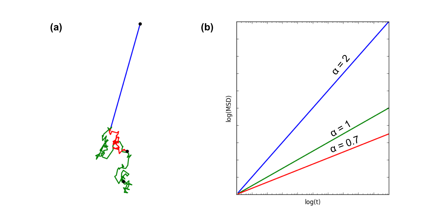
Figure 1: (a) Examples of trajectories of particles with ballistic (blue), diffusive (green), and subdiffusive (red) behavior. (b) The MSD for each trajectory on a log-log plot. An MSD with a slope of 2 or 1 indicates ballistic and diffusive behavior, respectively. An MSD with a slope smaller than 1 indicates subdiffusive motion.
To quantify the motion of 1 micrometer spheres in the mucus, the researchers track the motion of spheres in each mucus sample and calculate their mean square displacement (MSD). A particle’s mean square displacement describes how far it moves, on average, from its starting point in a given amount of time. The MSD is characterized by
$latex \langle r \left( t \right) ^2\rangle = 4 D_{\alpha} t^{\alpha}$
where $latex \langle r^2 \left( t \right) \rangle$ is how far the particle is from its starting point after t seconds and $latex D_{\alpha}$ describes how quickly the particle moves (called the diffusion coefficient). If a particle is acted on by a constant force, it moves in a straight line known as ballistic motion and $latex \alpha = 2$. This is not how a micrometer-scale particle in a fluid moves because it is being bounced around by random forces from the molecules in the fluid. Instead of moving in a straight line, the particle’s trajectory is a series of small excursions in random directions, and it takes longer to get away from its starting point than if it just moved in a straight line. This type of motion is known as free diffusion, and its MSD is characterized by $latex \alpha = 1$. In mucus, the polymer network gets in the way of the particle’s diffusion, so it can’t diffuse freely. This motion is called subdiffusive, and it has $latex \alpha < 1$. The more the particle’s diffusion is hindered by the polymer network, the lower its value of $latex \alpha$ will be. An example of a trajectory and MSD plot for each type of motion is shown in Figure 1.
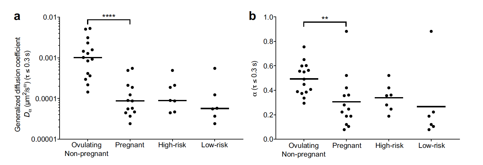
Figure 2: The diffusion coefficient $latex D_{\alpha}$ (a) and the diffusion exponent $latex \alpha$ (b) from the single particle tracking of 1 micrometer spheres in mucus samples. (Adapted from Smith-Dupont et al., 2017)
To compare the permeability of the mucus samples, the researchers measure $latex \alpha$ and $latex D_{\alpha}$ for each sample, as shown in Figure 2. The mucus from the pregnant women resulted in lower values of $latex \alpha$ and $latex D_{\alpha}$ than in the non-pregnant women, indicating that the network is more restrictive, as expected. However, the small difference between the high-risk and low-risk pregnancy women was not statistically significant [4]. This suggests that the difference in mucus permeability between high-risk and low-risk pregnancies is not primarily caused by differences in the mucus mesh size.
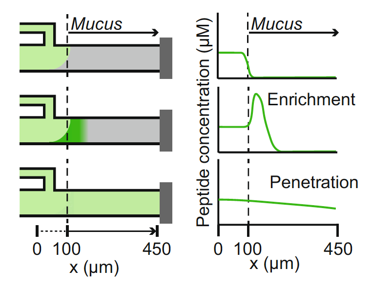
Next, the researchers look at the permeability of the mucus to small, fluorescently labeled peptides. They use a microfluidic device (to learn more about microfluidics, see [5]) to flow a solution of the peptides through the mucus, and observe whether the peptides get trapped or are able to flow through by looking at the fluorescent profile. Figure 3 shows a schematic of the microfluidic device. The ability of a small particle to travel through mucus is controlled by what happens when it comes in contact with part of the network. This interaction is thought to be affected by the charge of the particle, so the researchers investigate the behavior of both positively and negatively charged peptides.
Figure 3: A schematic of the microfluidic device used to determine the permeability of mucus samples to fluorescently labeled peptides. If the mucus is not permeable to the peptides they get stuck in the mucus, causing enrichment (or buildup) of peptides at the front of the mucus sample. If the mucus is permeable, the peptides penetrate the mucus and are seen throughout the sample. (Adapted from Smith-Dupont et al., 2017)
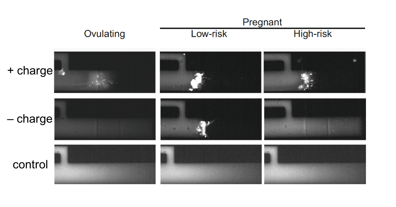
For both positively and negatively charged peptides, the researchers see a significant difference between low-risk and high-risk mucus, as shown in Figure 4. The mucus from both low-risk and high-risk patients was less permeable to the positively charged peptides than the mucus from the ovulating patients. However, more of the positively charged peptides were able to penetrate into the high-risk mucus than the low-risk mucus. The results for the negatively charged peptide were more dramatic. While the low-risk mucus was not permeable to the negatively charged peptide, the high-risk mucus was as permeable as that from the ovulating patients. This suggests that the biochemical properties of the cervical mucus in low-risk and high-risk patients are primarily responsible for differences in permeability.
Figure 4: Fluorescence profiles after 900 seconds for positively and negatively charged peptides through mucus samples. A control shows the profile in fluid with no mucin. (Adapted from Smith-Dupont et al., 2017)
The results in this study help to clarify which properties of cervical mucus cause an increased risk of preterm birth. The researchers considered both structural and biochemical origins for the increased permeability of cervical mucus to harmful pathogens. Structural changes in the mucin network do not appear to be the primary difference between cervical mucus in low-risk and high-risk pregnancies. Instead, biochemical changes in the mucus that affect how the mucus interacts with microbes appear to be the primary cause of its increased permeability in high-risk pregnancies. This understanding could be useful for developing diagnostic tools to determine a woman’s preterm birth risk and, ideally, treatment to reduce her risk.
[4] While the difference between high-risk and low-risk pregnant women is not significantly significant, this does not rule out a difference between the two. The sample size is relatively small for this study, with only 14 pregnant women (7 low-risk and 7 high-risk) included, so the lack of statistical significance could also be due to insufficient data.
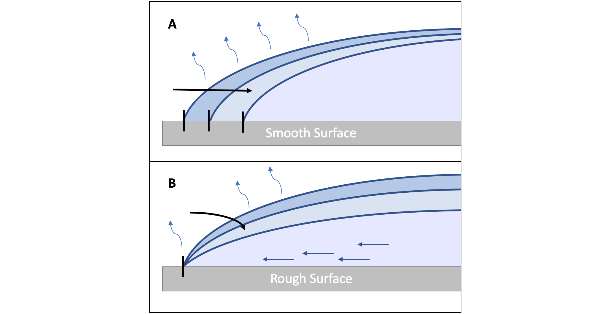
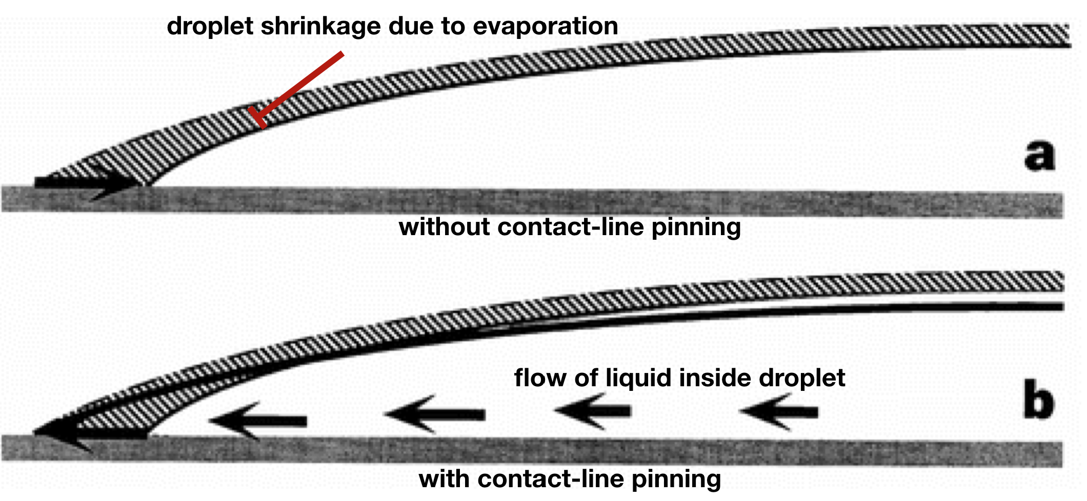
When I first learned about the coffee ring effect I thought it was super cool, but it seemed like an open-and-shut case. Why do rings form where some liquids, like spilled coffee, are left to dry? Roughness on the table causes the liquid to spread imperfectly across the surface, pinning the edges of the droplet in place with a fixed diameter. Because the diameter of the droplet can’t change during evaporation, new liquid must flow from the droplet’s center to the edges. This flow also pushes dissolved coffee particles to the edges of the droplet, where they are left behind to form a ring as the water evaporates away (Figure 1). More details can be found in our previous post, here. It’s a complicated phenomenon, but after being described in 1997 it doesn’t seem like anything new would be going on here. Right? Well, as usually happens in science, classic concepts have a way of popping back up in unexpected ways. Last year It?r Bak?? Do?ru and her colleagues in Prof. Nizamo?lu’s group at Koç University, Turkey published a study using the often troublesome coffee ring effect to their advantage: making self-assembling silk lasers.
Figure 1: Pinning and the Coffee Ring Effect. A cross section of a water droplet drying on a smooth surface (A) versus a rough surface (B). On a smooth surface the droplet shrinks due to evaporation. On a rough surface the edge of the droplet is pinned and cannot shrink, forcing an internal flow to maintain the droplet’s shape.
The fundamentals here are the same as the classic coffee ring effect, but instead of coffee particles Do?ru’s droplets hold a colloidal suspension of silk fibroin proteins. In a colloidal suspension, particles (such as proteins) are mixed in another material (such as water) and neither dissolve fully into solution nor precipitate out. Smoke, milk, and jelly are all examples of colloids. Harnessing the coffee ring effect to build 2D structures out of colloidal particles has been well developed since Witten’s description of the coffee ring effect in 1997 [1], but 3D self-assembly is much less common. What makes Do?ru’s 3D structures possible is the fibroin protein.
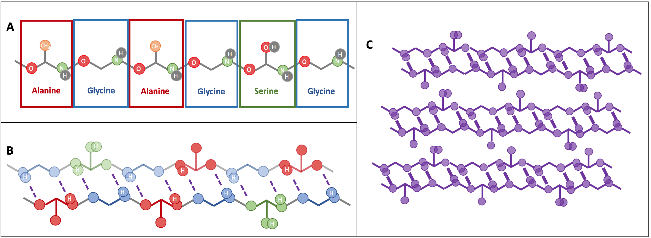
Fibroin is the primary component of silk from the silkworm Bombyx mori. These fibers have been used by humans for thousands of years to make textiles, but recently the fibroin protein has taken on new life when extracted from silk as an aqueous, water-based, suspension and regenerated into other forms [2,3]. Fibroin proteins are long, and they easily tangle up and bond to each other to form networks of layered crystalline structures called beta-sheets (?-sheets) (Figure 2). These sheets give silk fibers and other fibroin materials strength and toughness. Furthermore, fibroin materials are biocompatible and biodegradable.
Figure 2: Silk Fibroin And ?-sheets. Silk is made of long fibroin proteins (a) that have a repeating molecular structure. These proteins bond together into ?-sheets (b), which then stack together (c) to form materials with high strength and toughness.
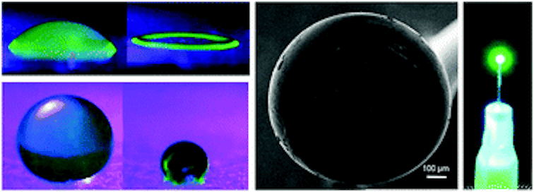
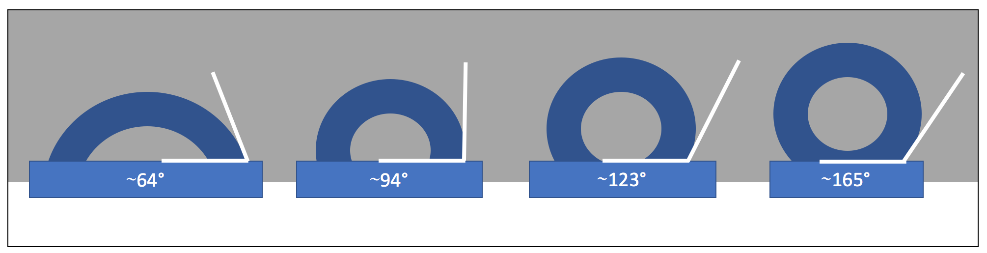
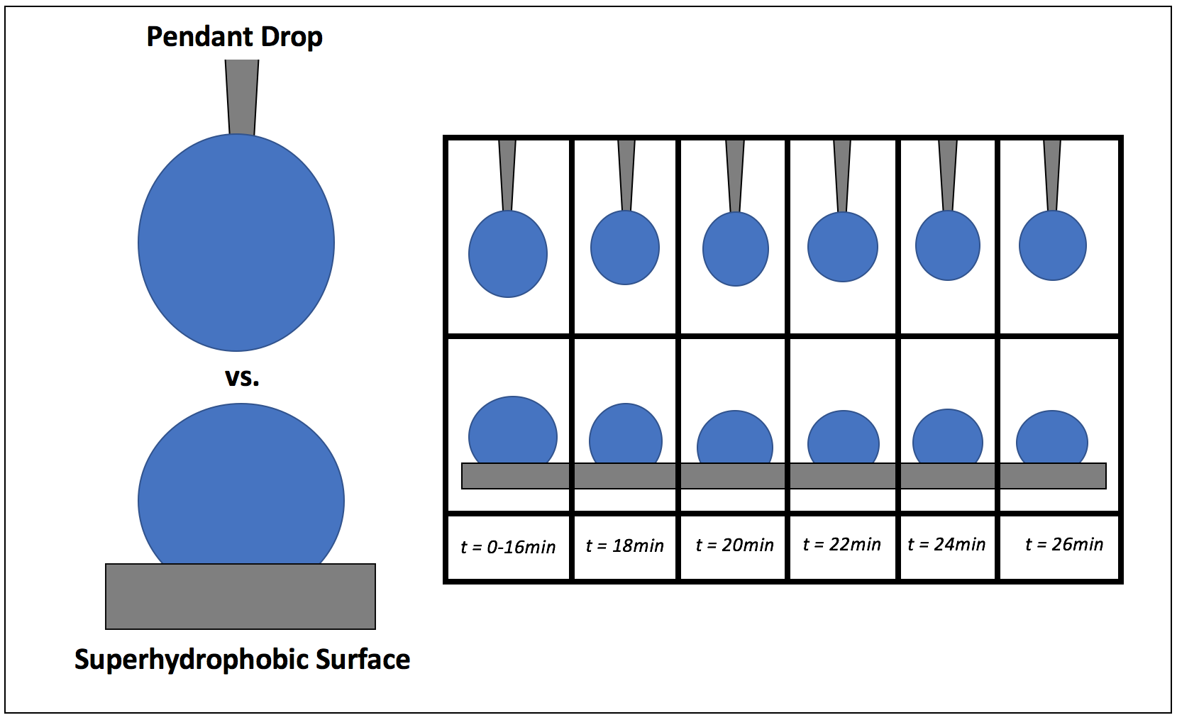
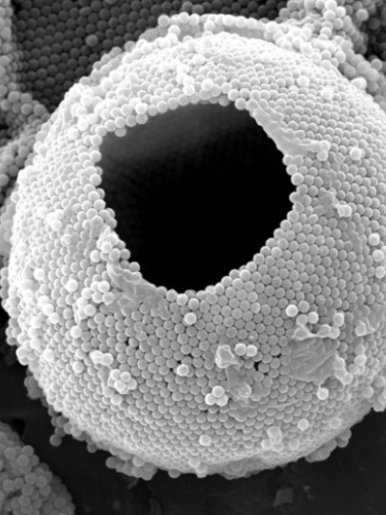
To create 3D structures with the coffee ring effect, Do?ru, Nizamo?lu, and their coworkers put droplets of silk solution on superhydrophobic surfaces. Superhydrophobic surfaces strongly repel water, preventing water-based liquids from spreading flat across the surface and making the droplets stand straight up during the drying process. This makes the angle between the edge of the droplet and the surface (called the contact angle) particularly high, between 95-145 degrees throughout evaporation. The interaction between water and the superhydrophobic surface determines the shape of the final structure, with high contact angles creating more spherical droplets (Figure 3). After a solid 2D ring of fibroin forms on the bottom, the silk proteins continue to stack along the droplet’s surface, forming a stable spherical shell of ?-sheets that the remaining water can evaporate through. The researchers found that the concentration of the fibroin solution was important for controlling the final structure. If the solution is too dilute then the shell will collapse in on itself, but if the fibroin concentration is too high the initial contact angle will be lower and the final structure will also be more 2D than 3D.
Figure 3: Contact Angle. Droplets of the same solution show different contact angles on different surfaces (as adapted from Do?ru’s paper). On the left is a mildly hydrophobic surface, and on the right is a superhydrophobic surface. Note how the size of the contact angle (shown in white) increases with the hydrophobicity of the surface.
To make 3D spheres, the researchers tried the pendant drop method, hanging a droplet from the tip of a needle. Similar to getting high contact angles from a droplet on a hydrophobic surface, hanging a droplet from a needle gives that droplet a small contact area, and a spherical shape (Figure 4). If the diameter of the needle is the same size or smaller than the contact area of the droplet on a superhydrophobic surface, then the shape of a droplet squeezed out of the needle should be as or more spherical than the droplets in the previous experiment. In this study, the pendant drop method ends up producing more uniform drying. These pendant-drop shells are smooth enough inside to act as optical resonators, surfaces that reflect light waves back on themselves so the waves amplify each other (the “a” in “laser,” which I always forget comes from the acronym for “light amplification by stimulated emission of radiation”).
As a proof of concept, the researchers made shells out of fibroin mixed with green fluorescent protein (GFP). Fibroin ?-sheet formation is so stable that it still happens when small amounts of other materials are present, so the optical resonator can form in the same way it did with a fibroin-only solution. In this case, because GFP has been added, when the structure is exposed to the right light source it will amplify green light emitted by the shell itself – an “all protein laser” in the making.
Figure 4: Benefits of the Hanging Pendant Drop. The hanging pendant drop method can produce similar spherical drops to a hydrophobic surface. It was shown that the pendant drop method produces more spherical final structures (adapted from Do?ru’s paper).
Part of what’s exciting about this publication is that the authors harness the coffee ring effect for a fun new type of small scale, self-directed 3D “printing.” They showed that the method works for other polymers as well, but I agree with their choice to highlight the silk protein fibroin. Not only is fibroin biocompatible, but it also has the potential to be more environmentally friendly to process than other polymers and is already produced in large quantities globally as part of the textile industry.
[1] Han, W. and Lin, Z. “Learning from ‘Coffee Rings’: Ordered Structures Enabled by Controlled Evaporative Self-Assembly.” Angew. Chem. Int. Ed. 51 (2012): 1534–1546.
The skeleton is the backbone of the body, both literally and figuratively. Healthy bones protect soft organs from injury and enable the body to move. Starting from childhood, staying active and following a healthy diet helps the body maintain healthy bones. However, as people age, their bones can start to weaken. There are often no early symptoms to weakening bones, and as a result the first indication of a problem may be a painful break once the weakening has already significantly progressed.
Although it may seem like bones are made of a hard material, they are actually an elegant combination of hard and soft materials. A primary component of bone is collagen, which forms a soft protein network. This network then provides a scaffold for calcium phosphate, a mineral that provides bone with its hardness and strength. This mixture of hard and soft material enables bone to be flexible enough to withstand impacts, but rigid enough to maintain its structural integrity.
Bone tissue, like other tissue in the body, is alive and therefore able to grow and heal. The material in bones is always being resorbed (or removed) by the body and simultaneously replaced. Around the age of thirty, the rate of resorption overtakes the rate of replacement, causing bones to slowly weaken. When these rates become too disparate, osteoporosis can develop, causing bones to become weak and porous [1].
Bone fractures are more common in patients with osteoporosis, and when they occur, treatment is often needed at the site of the break to promote bone regeneration. The typical treatment in these cases is an autologous bone graft, which involves taking bone from another area in the patient’s body and transferring it to the fracture site to help promote bone regrowth. This technique has two clear downsides: there is limited availability of bone tissue for grafting since it has to come from somewhere else in the person’s body, and removing bone tissue for a bone graft can cause damage to the donor site.
As a result, researchers are working to develop synthetic materials that can provide a better alternative to autologous bone grafts. A promising material would promote bone growth and be strong enough to sustain bending and support weight. Additionally, it needs to be non-toxic and not cause an immune system reaction. Synthetic bone graft materials already exist, but they do not work as well as bone grafts taken from the patient’s own body because they are not as mechanically strong and they do not promote as much bone growth. Hence, the search for better synthetic bone graft materials continues.
In today’s paper, Mani Diba and co-workers investigate a new synthetic material for use in the regeneration of bone tissue in osteoporotic patients. The material in question is a colloidal gel, which is a disordered network structure made of microscale particles suspended in a liquid. This network allows the material to resist applied forces and behave like a solid, even though it may be mostly made up of liquid. Colloidal gels are different from chemically covalent bonded gels [2], like jelly or agar, because their building blocks are microscale particles instead of polymers. These particles bond to each other mostly because they are hydrophobic, or water-repellent, so they would prefer to be next to each other than surrounded by water. The bonds between the colloidal particles are reversible, meaning they can break and reform more easily than covalent bondsin polymer gels, which allows the colloidal gel network to be more adaptable and reform after being broken apart.
The behavior of the colloidal gels is similar to that of toothpaste, which acts like a fluid as it is being forced out of the tube, but once it stops being squeezed it becomes more solid again and doesn’t flow off your toothbrush. For a bone graft material, this means that the colloidal gel can behave as a liquid as it is being injected into a bone defect, and then harden as the network reforms once it’s in place. While this is not a requirement for bone graft materials, it does make the material easier to put in place at a bone defect site.
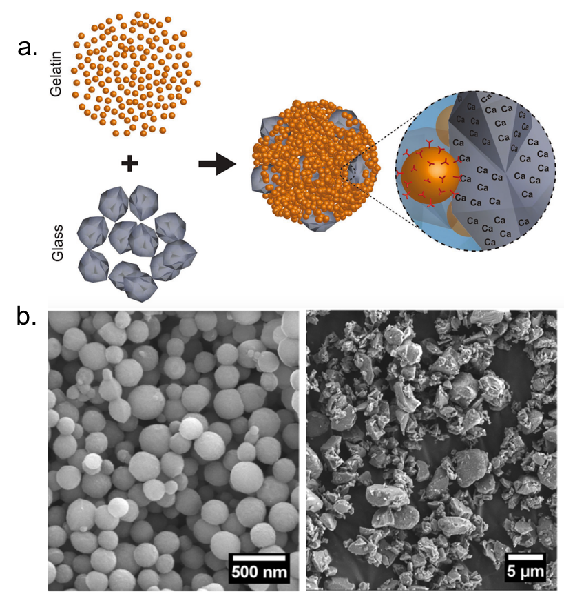
The researchers prepare a colloidal gel by mixing gelatin particles and glass particles in water (see Figure 1). This choice of particles mimics the structure of bone tissue by using gelatin- a soft material- with glass, which is hard and provides mechanical strength. In order to be a good replacement for a bone graft, the gel must satisfy two main requirements. First, it needs to be mechanically robust to serve as a load-bearing scaffold for bone growth. Second, it needs to be biocompatible, meaning that it should support the growth of new bones.
Figure 1: (a) A schematic showing the formation of a gel by mixing glass and gelatin particles (b) Electron microscopy images of colloidal gelatin (left) and glass (right) particles (adapted from Diba et al.)
The first set of experiments in this paper look at the mechanical properties of the colloidal gel by measuring its storage modulus, which characterizes how strong the gel is. The researchers find that increasing the ratio of glass to gelatin particles or increasing the total number of particles in the gel increases the storage modulus by a factor of more than 100, from about 0.1 kilopascal to tens of kilopascals. The gel is also able to recover its initial storage modulus after being broken apart by shearing, similar to how silly putty can recover its mechanical properties after being stretched. This indicates that the network is able to reform in the bone and become solid again, as expected.
After characterizing the gel’s mechanical properties, the researchers investigate whether it can promote new bone growth. The growth of new bone starts with the multiplication of osteoblasts, or bone-forming cells, that produce bone matrix material. A signature of this process is an increase in the levels of certain enzymes. Once the matrix is well formed, it undergoes mineralization, which is the deposition of inorganic material (calcium) onto an organic matrix (collagen). This process can be monitored by measuring the amount of calcium added to the area [3]. The researchers track these two indicators, enzyme levels and calcium deposition, to measure the biocompatibility of the gels.
Diba and coworkers study the biocompatibility of the gels both in test tubes and in living animals. In the test tubes, they only find significant mineralization at a glass to gelatin ratio of 0.5 (the highest investigated), which also corresponds to the largest peak in enzyme levels. For testing in animals, the researchers therefore opt for a composite gel with a glass to gelatin ratio of 0.5 and compare the bone growth to that with a single-component gel with no glass particles. The researchers implant these gels in bone defects in the femurs of osteoporotic rats and measure the amount of bone growth after 8 weeks.
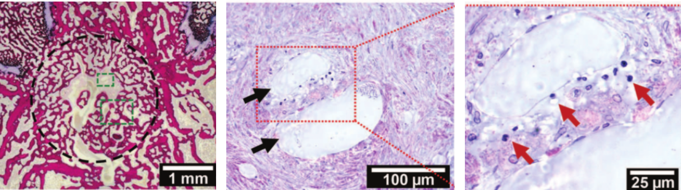
Surprisingly, in the rats, the addition of glass particles to the gel did not increase the amount of bone mineralization beyond that seen in the single-component gel as the researchers hoped. However, the bone growth in the composite gel did show more blood vessel-like structures than in the single component gels (see Figure 2), which is important because bone—like other living tissues—needs blood flow to supply oxygen and nutrients, as well as to remove waste products.
Figure 2: Images of bone regrowth from the composite gel in a rat femur. Left: Bone regrowth in a defect that was originally the size of the black circle. Center: Higher magnification image of the small green rectangle on the left. Black arrows point to blood vessel-like structures. Right: Higher magnification of the red rectangle in the center. Red arrows point to cells observed in the center of the original defect. (Adapted from Diba et al.)
Though the researchers in this study did not find the desired increase of bone mineralization in live rats by using a composite gel instead of a single-component gel, they did see other indicators of improvement. Including glass particles increased the storage modulus of the gel, indicating more mechanical strength. They also saw indicators of improved biocompatibility. The bone growth in the composite gel showed an increase in blood vessel-like structures, and they found test tube results which suggested that including the glass particles may still improve mineralization if a higher ratio of glass to gelatin is used. Considering these improvements over a single-component colloidal gel, this composite colloidal gel is a promising development in the search for better bone graft materials.
[2] Covalent bonding is the sharing of valence electrons, which are in the outer shell of electrons, between atoms to make a full valence shell. Any time two non-metals come together they will share their valence electrons.
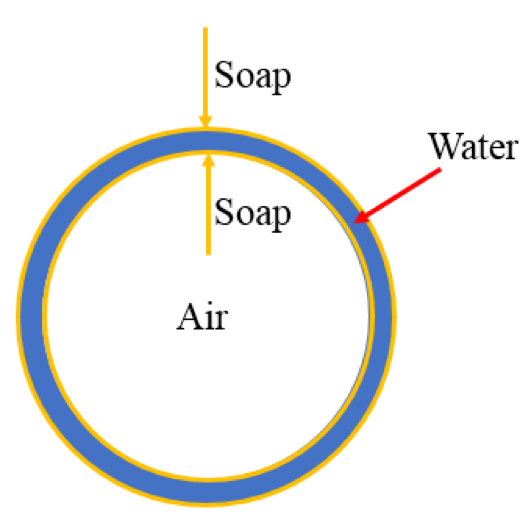
Most of us have had the childhood experience of blowing bubbles. But have you ever wondered how bubbles form and what keeps them stable? The key to making bubbles is surface tension, the tension on the surface of a liquid that comes from the attractive forces between the liquid molecules. Water has a very high surface tension (that’s why bugs can walk on water) making it difficult to stretch to form a thin water layer that we see when bubbles form.By adding soap to water, we can lower the surface tension of the water, allowing us to stretch this water-air interface to form a thin water sheet. As you blow more and more air into a bubble, the bubble will grow larger and larger as the thin layer stretches. Eventually, you’ll reach the limit of the added stretchiness, and the bubble will burst, engraving in your memory its fragile nature.
A typical air bubble made out of a water-soap mixture (Figure courtesy of Gilad).
In soft matter, sometimes scientists utilize materials such as solid macroscopic particles instead of soap molecules to reduce the surface tension of an interface. Using particles to stabilize an interface allows them to tailor the mechanical and chemical properties of the interfaces to fabricate capsules. For instance, if a capsule needs to travel in blood-stream for therapeutic purposes, it must be tough enough to withstand blood pressure without rupturing. But if we make such a capsule how can we measure its mechanical response?
In this post, we’ll look into the work by Niveditha Samudrala and her colleagues on measuring the mechanical properties of a particle-stabilized interface. They utilize a direct approach of applying force on such a stabilized interface to study its mechanical response that has eluded earlier techniques. Knowing the stiffness of these particle-coated interfaces, say in the form of capsules, would enable us to use them for different controlled-release applications such as treating a narrowing artery [1] as well as tune them to have different flow properties.
The authors use tiny (smaller than a micrometer!) dumbbell-shaped particles with different surface properties to stabilize an oil-in-water emulsion (see note [2]). Here instead of a thin layer of water sandwiched by the soap molecules, the water-oil interface has been stabilized with micron-sized particles. This stabilization technique will render higher mechanical properties to the interface. Droplets stabilized in this way, known as colloidosomes, have been shown to be capable of encapsulating a wide variety of molecules.
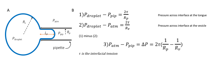
The researchers characterized the particle-stabilized droplets using the micropipette aspiration technique. To understand this technique, imagine picking an air bubble with a straw. What you need to do is to approach the air bubble and then apply a gentle suction (or aspiration) pressure. When the suction pressure becomes larger than the pressure outside of the droplet, then the droplet gets aspirated into the straw forming theaspiration tongue (Figure 1A). Similarly, in the micropipette aspiration technique, a glass pipette (the straw) with an inner diameter of $latex R_p$ is usually used to aspirate squishy stuff, such as cells, vesicles, and here droplets.
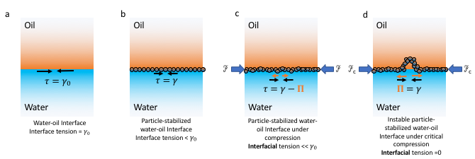
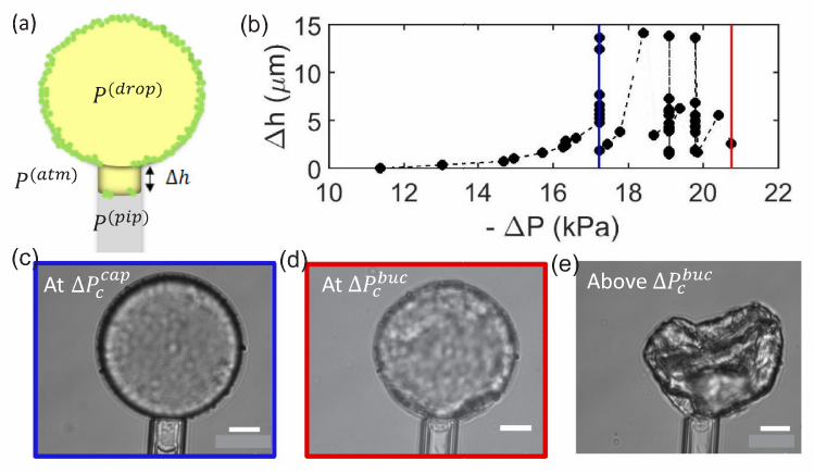
To obtain the tension response, therefore the toughness of an aspirated interface, we need to consider the pressures applied to the interface. Let’s consider an aspirated droplet as shown in Fig 1A at mechanical equilibrium (which means the sum of all the forces is zero). We know that each interface has a surface tension acting on it (See Fig 2a). In our bubble example, I mentioned that the soap molecules tend to gather at such interface to decrease the tension (See Fig 2b). But when there are other forces acting on the interface in addition to the presence of the molecules, such as the suction pressure in our case, the tension of the interface now comes from both the surface tension and the suction force. We call this total force the interfacial tension (See Fig 2c). The Young-Laplace equation can be used to relate this interfacial tension to the pressure applied to the interface (Fig 1-B3).
Fig1. Schematic representation of the aspiration technique (A) and the Young-Laplace equations obtained at both interfaces of the outer edge of droplet and tongue inside the pipette (B). $latex P_{atm}$ is the atmospheric pressure set to zero, $latex P_{droplet}$ is the pressure inside the droplet. $latex P_{pip}$ is the suction pressure. $latex R_{v}$ is the radius of droplet outside the pipette and the $latex R_{p}$ is the pipette radius.
When the molecules, or particles in our case, are forced to pack tightly together they oppose the compression force. This opposition is felt at the interface by a pressure called surface pressure (see Fig 2c). Under the interface tension and the surface pressure, the new net interfacial tension is defined as:
$latex \tau=\gamma_{0} – \Pi$.
where $latex \Pi$ is the surface pressure, $latex \gamma_{0}$ is the interface tension which is constant for a given interface.
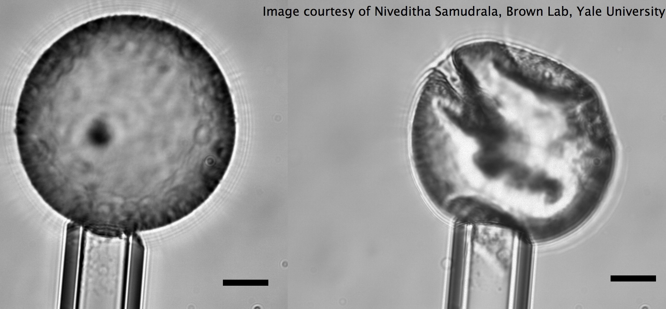
In this study, Samudrala and her colleagues show that there are two critical pressures after which instabilities form at the interface resulting in droplet dripping into the pipette and buckling respectively (Fig 2d). They conclude that the dripping happens due to the transition of the interface from a particle-stabilized interface to a bare oil-water interface resulting in a sudden suction of tiny oil droplets (basically the droplet drips at this point, see Fig 3B, blue and 3C).
The second instability is the buckling which the researchers propose happens when $latex \tau$ tends to zero. Now let’s see how buckling happens.
Fig 2. The schematic of a particle-stabilized water-oil interface under different load is shown. (a) shows the bare water-oil interface. This interface has a constant, material related surface tension, the $latex \gamma_{0}$. (b) depicts a particle-coated interface. The aggregation of the particles at the interface, decrease the interface tension to a new value of $latex \gamma$. (c) the particle-coated interface is compressed from both ends. This case happens in our case when the particle-coated droplet is stretched (see the text). (d) the compressed interface reaches a critical pressure upon which the net tension of the interface is zero and the buckling happens as the interface cannot no longer endure the imposed force.
The dripping at the first critical pressure decreases the volume of the particle-coated droplet, but note that the surface area is constant because neither particles leave the surface nor the free ones join the droplet (the latter argument is assumed). The continuation of the increase in suction pressure plus the volume lost in the dripping step results in the buckling of the interface (Fig 3b red and 3E, also see note [3]). When the authors aspirate the bare oil droplets as well as droplets stabilized by small molecules, they only see the sudden droplet disappearance with no shape abnormalities due to the fluid nature of the interface rather than solid-like nature for the particle-stabilized case. But why does the buckling happen?
Fig 3. Evolution of instabilities of a particle-coated droplet under tension. (a) shows the schematics of the particle-coated droplet being aspirated. (b) Change in aspiration length as a function of suction pressure. Blue line remarks the capillary instabilities. Red line shows the elastic failure of buckling process. (c & d) are the images of capillary and buckling instabilities respectively. (e) shows the case when the suction pressure is above buckling pressure at which the particle coat fails (the figure is adapted with no further change from the original paper).
Recall how we defined the net interfacial tension above; $latex \tau=\gamma – \Pi$. The authors hypothesize that upon suction of a particle-stabilized droplet, particles jam at the interface of the droplet outside of the pipette, creating a high surface pressure. When this surface pressure approaches $latex \gamma$, the net tension becomes zero ($latex \tau=0$, see fig 2d and note how the interface tension is opposed by the surface pressure due to repulsion between particles). When an interface possesses no tension, it means that the interface can no longer bear any loads. Considering any sort of defects or irregularities due to nonuniform particle packing, for such interfaces deformations such as buckling will form. Now, let’s see how the authors test their hypothesis.
The authors observed that at the tip of the tongue, there is a very dilute packing of particles in such a way that the interface to a good approximation resembles the Fig 2a, a bare water-oil interface. With this observation, one can safely assume that the interfacial tension, the $latex \tau$ is equal to the oil/water interface tension, the $latex \gamma$ and write the Young-Laplace equation across the tip of the tongue (see Fig 1B-(1)):
where $latex R_{p}$ is the radius of the pipette and is fixed. The authors experimentally show that for a range of droplet size ($latex 10\ \mu m < R_{droplet} < 100 \ \mu m$), the droplet pressure right before buckling varies very close to zero (in above equation all parameters are known except the $latex P_{droplet}$, which is calculated when we put $latex P_{pip} = P_{buckling}$). Therefore, considering the equation (2) in Fig 1B, the net tension would be zero (see note [3]) and with this, the authors correlate that the reason for the formation of buckling is the net-zero tension of the interface.
Taking it all together, we saw that for a droplet with solid-like thin shell, the mechanical response is completely different from the bare or the molecule-stabilized interface. A fairly rigid interface undergoes buckling due to its net tension tending to zero and knowing the threshold of buckling will enable us to tune the mechanical properties of such droplets for different applications from load-caused cargo release (see note [1]) or emulsions with varied flow properties. Imagine if we encapsulate a fragrance in our air bubble, which upon rupturing will release the scent. Now, wouldn’t it be nice if we could control the toughness of this bubble or similar architecture to rupture under a specific condition that we desire (see note [1])?
[1] In a disease called atherosclerosis, the arteries narrow down due to plaque buildup. In this narrow region, the blood pressure is higher than the normal region of the artery. So one can use this pressure difference to crack release the relevant drug from the capsule only in the narrow regions of the artery to dissolve the plaques away. Neat!
[2] If we apply a shear force on a mixture of two or more immiscible liquids in the presence of a stabilizing agent, we produce an emulsion and the stabilizing agent is called an emulsifier. The particles show a significantly higher tendency to gather at an interface in comparison to amphiphilic molecules. Thus, particles are strong emulsifiers. If we mix lemon juice and oil, soon after stopping the mixing, the two solutions will separate. Now, if you add eggs, you stabilize this mixture (egg works as an emulsifier) and you get Mayonnaise!!
[3] The authors report that for particle-stabilized droplets they observed different deformation morphologies such as wrinkles, dimples, folds and in some case complete droplet failure. They attribute this diversity to the non-uniformity of particle packing at the interface. But what is interesting to me is when they decrease the suction pressure, the droplets go back to their original spherical shape and then upon the second aspiration, the deformations happen at the same exact location as were for the first aspiration. This means that during the suction, there is limited particle rearrangement (Watch here).
[4] We can easily set the atmosphere pressure to zero before aspirating the droplets, thus here the $latex P_{atm} = 0$.
Figure 1. A 2-cm dried drop of coffee with a stain around the perimeter, forming a coffee ring. Adapted from Deegan et. al.
I’ve spilled a lot of coffee over the years. Usually not a whole cup, just a drop or two while pouring. And when it’s just a drop, it’s easy to justify waiting to clean it up. When the drop dries on the table, it forms a stain with a ring around the edges (Figure 1), giving it the look of a deliberately outlined splotch of brown in a contemporary art piece (when I say “coffee ring” I mean the small-scale, spontaneously formed stain around the edge of the original drop, rather than the imprint left on a table from the bottom of a wet coffee cup). But the appearance of these stains is simply a result of the physics happening inside the drop. Coffee is made of tiny granules of ground up coffee beans suspended in water, so the ring must mean that these granules migrate to the edge of the droplet when it dries. Why do the granules travel as they dry? Today’s paper by Robert D. Deegan, Olgica Bakajin, Todd F. Dupont, Greb Huber, Sidney R. Nagel, and Thomas A. Witten provides evidence that coffee rings arise due to capillary flow–the flow of liquid due to intermolecular forces within the liquid and between the liquid and its surrounding surfaces.
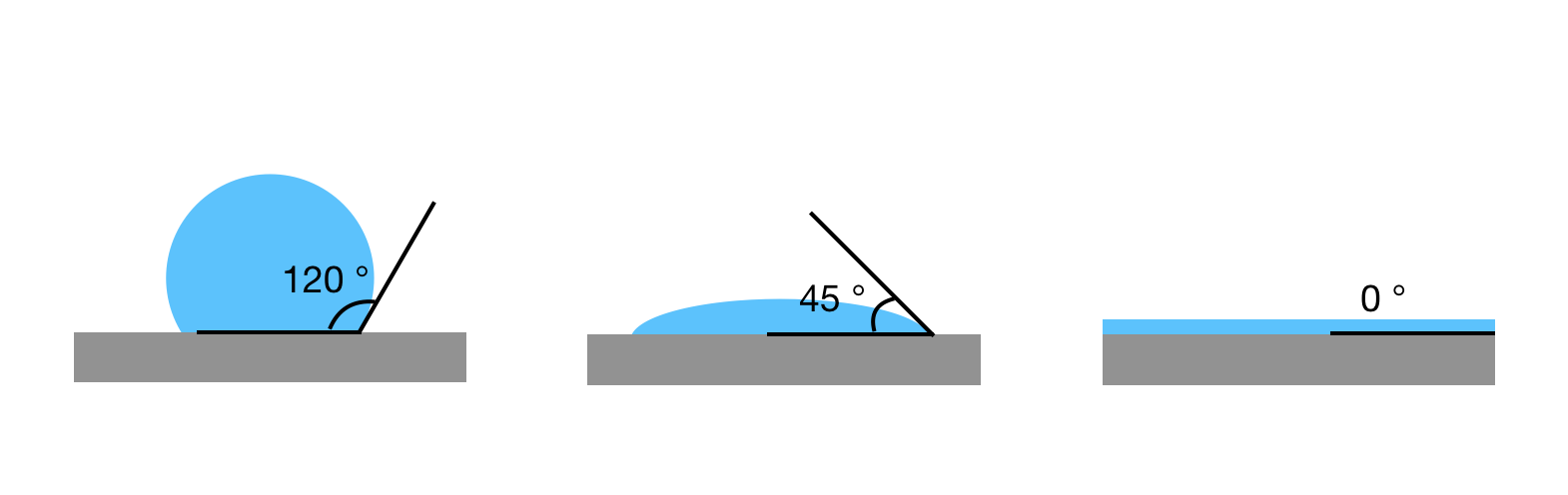
Figure 2. Diagrams of contact angles for different droplets. From left to right, the first is exhibits poor wetting, with a large contact angle. The next has good wetting, with a smaller contact angle. The last has perfect wetting, with a contact angle of zero, and coffee grains suspended in this solvent would not be able to form a ring upon drying.
The researchers found that these rings don’t just form in coffee. Their observations showed that the rings form in a wide variety of solutes (the suspended coffee granules), solvents (the water), and substrates (the table you spill on) as long as a few conditions are met. First of all, the droplet has to have a non-zero contact angle[1] (See Figure 2). In other words, the droplet doesn’t spread out into a completely flat puddle on the table. Second, the contact line has to be pinned. This means that the surface has irregularities or roughness that cause the edge of the droplet to get stuck in place. Last, the solvent has to evaporate; the ring won’t form if the droplet never dries.
So now we know the conditions required for rings to form, but we want to know how they form. Deegan and his colleagues found that the rings are caused by a geometrical constraint. Here’s how it works: The pinning of the contact line means that the perimeter of the droplet cannot move, so the diameter of the droplet has to remain constant. But if the water in the droplet is evaporating, the droplet’s height will be reduced at every point (Figure 3a). Along the edges, where the droplet is thinnest, the height would be reduced to zero, and the droplet would shrink.
But the contact line pinning means that droplet can’t shrink. To prevent this shrinkage, liquid must flow out to replenish the liquid at the droplet edge as it evaporates. This flow brings with it the suspended coffee granules (or whichever solute is suspended in the solvent), pushing them outward until they pack at the edge of the droplet to form a ring (Figure 3b).
Figure 3. (a) Diagram showing the cross-section of a droplet on a surface. The shaded region shows how the droplet will shrink due to evaporation after a small amount of time if the contact line is not pinned. (b) Now, a black line is added to show how the droplet will shrink if the contact line is pinned. The arrows indicate that more liquid must flow to the outside of the droplet to replace what is lost to evaporation. Adapted from Deegan et. al.
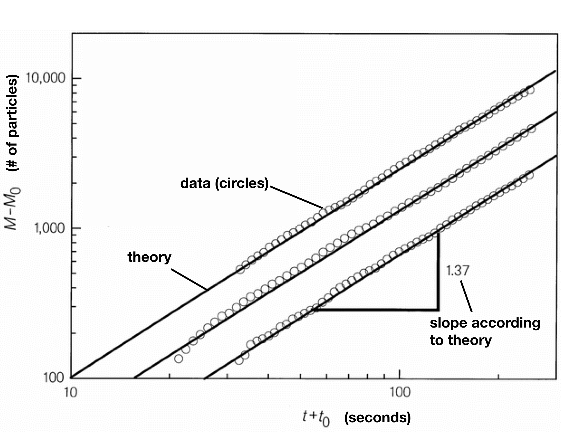
By calculating how quickly water evaporates from the surface of a droplet, the researchers derived an expression for the mass of the ring as a function of time. It takes the form of a power law, which can be shown as a straight line on a log-log plot. Equipped with a quantitative prediction, the researchers set about performing experiments to test their model. Instead of using coffee, they opted for plastic microspheres suspended in drops of water. They placed the drops on glass slides and used a video microscope to image the droplets as they dried, recording the particles moving to the edges of the droplet (Figure 4).
Figure 4. Particles flowing to the edge of a droplet during evaporation to form a ring. Video from [2] and produced by Deegan et. al.The researchers knew the mass of the individual particles, so they were able to calculate the mass of the ring as a function of time by counting the particles as they traveled to the edges. The results were shifted by an offset time t0 to account for early times where the power law prediction doesn’t hold and were shifted by mass M0 to account for the particles deposited during this initial stage. From the plot comparing the data and theory (Figure 5), we can see that the prediction shows good agreement with the data.
Figure 5. Plot of mass in the ring as a function of time. The mass is plotted in units of particle number, so the plot shows how the number of particles grows over time. The three lines correspond to three different droplets. The upper curve overlapped with the middle so was shifted up for clarity. The circles show data and the solid lines show the theoretical prediction. The slope of 1.37 is the exponent of the power law predicted by the theory; On a log-log plot, a power law is a line with the exponent as the slope. Adapted from Deegan et. al.
In the twenty years since this paper was published, the study of drying droplets has continued in full force [3]. Scientists have discovered various particle patterns that can form under different drying conditions. Why do we care so much about these drying droplets? If the beauty of the physics isn’t motivation enough, then maybe the applications will convince you. The physics of drying is essential to inkjet printing, and a better understanding of the drying process could help make more precise printers [4]. Drying patterns can be used to identify the presence of certain proteins, making this a potential tool for disease detection [5]. Maybe next time you spill some coffee, you’ll take a moment to think of the physics of the drying droplet before you wipe it away.
[1] The contact angle is the angle where a liquid-gas interface meets a solid surface. The smaller the contact angle, the better the wetting of the surface.
Disclosure: The first author of the article discussed in this post, Anthony Dinsmore, is now my Ph.D. advisor. He did his postdoc at Harvard University a while ago, and consequently, I was never involved in this work.
In past two decades, several approaches have been developed and optimized to encapsulate a wide variety of materials, from food to cosmetics and the more demanding realm of therapeutic reagents. Inspired by biological cells, the first attempts were to use either natural or synthetic lipid molecules to form encapsulation vessels, the so-called liposomes. Then, with the increasing awareness of controlled release of cargo, especially for therapeutic purposes, advanced materials such as polymers were developed to form carrying vessels. There has been an enormous progress in encapsulation technologies, however, these methods can be limited in their applicability regarding encapsulation efficacy, permeability, mechanical strength, and for biological applications, compatibility. In this article, Anthony Dinsmore and his colleaguesintroduce a new platform and structure to encapsulate almost all types of materials with finely controlled and tuned properties.
Colloidosomes
An emulsion is produced typically by application of a shear force to a mixture of two or more immiscible liquids like the classical water-oil mixture. The resulting solution is a dispersion of droplets of one liquid in the other continuous liquid. In such case, an interface between the fluids exists that would impose an energy penalty on the system. Therefore, the system will always attempt to minimize it, in essence by reducing the area of the interface that is to merge the similar liquid droplets. Amphiphilic molecules are known to segregate in such interface to further reduce the energy and to inhibit the merging of droplets. This segregation is not limited solely to molecules though. Solid particles tend to jam in the interface for the same reason to stabilize the emulsions. Inspired by the idea of particle-stabilized emulsions, which are known as Pickering emulsions, Dinsmore, and his colleagues have developed capsules made of solid particles. They adopt the name “Colloidosomes” by analogy to liposomes and demonstrate how the arrangement of these particles can be manipulated and controlled to achieve a versatile encapsulation platform.
Fabricating the Capsules
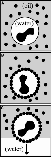
Colloidosomes are prepared first by making the emulsion in which the continuous phase contains the particles. For instance, in water-in-oil emulsions (“w/o”), water droplets become the core of the colloidosomes and particles are dispersed in the oil phase. Gentle agitation of such system results in particles being trapped in the water-oil interface (see Fig.1). The authorssummarize the capsule formation in three main steps:
Fig 1. The colloidosome formation process is illustrated schematically in three steps. (A) a water/oil emulsion first is created through gentle agitation of the mixture for several seconds. (B) Particles are adsorbed to the w/o interface to minimize the total surface energy. Through sintering, van der Waals forces, and or addition of polycations ultimately the particles are locked in the interface. (C)In the end, the particle-stabilized droplet is transferred to water via centrifugation.
(a)Trapping and stabilization. When the water-oil interface energy surpasses the difference between particle-oil and particle-water interface energy, particles are absorbed to the water-oil interface and become trapped due to the presence of a strong attractive well. This differs substantially from the case where particles were adsorbed to the interface via electrostatics, which requires the droplets to be oppositely charged to attract the particles. The packing of the particles at the interface is adjusted by controlling their interactions. Typically, the electrostatic interaction between particles, due to their surface chemistry, is utilized to stabilize the packing of the particle. For instance, in this study particles are coated with a stabilizing layer which in contact with water turns into a negatively charged layer.
(b)Locking particles. To form an elastic and mechanically robust shell, the particles must be locked in the interface. This results in an intact capsule that can withstand mechanical forces. One way to obtain such elastic shell is to sinter the particles in place. Sintering is a thermally activated process in which the surface of particles melts and connects them to each other. Upon this local melting, the interstices among particles begin to shrink. With longer sintering times, it is possible to completely block the interstices, which results in very tough capsules with extremely high rupture points. In this study, particles with 5 minutes of sintering yielded a 150 nm interstices size, and with 20 minutes, almost all the holes were blocked. By using particles with different melting temperatures, the sintering temperature can be adjusted over a wide range; this might be advantageous for encapsulants incompatible with elevated temperatures. Other ways of locking particles are electrostatic particle packing and packing via van der Waals forces. In the former case, for instance, a polyelectrolyte of opposite charge can be used to interact with several particles to lock them in place. In the latter case, for the van der Waals force to be effective, the steric repulsions and barrier must be destroyed so the surface molecules can get close enough for the London forces [1] to be strong.
After the Colloidosomes are formed, through gentle centrifuging, the fluid interface can be removed by exchanging the external fluid with one that is miscible with the liquid inside the colloidosome. In this step, having a robust shell to withstand shear forces crossing the water-oil interface is very important. This process ensures that the pores in the elastic shell control the permeability by allowing exchange by diffusion across the colloidosome shell. Now, with these steps and knowing parameters such as surface chemistry and locking condition, a promising system with characteristic permeability or cargo release strategies can be designed.
Tuning Capsule Properties; Permeation and Release
The most important feature of a colloidosome, as a promising encapsulant, is the versatility of permeation of the shell and or the release mechanisms. Sustained release can be obtained via passive diffusion of cargo via interstices that can be tuned via particle size and the locking procedure. With the mechanical properties of capsules optimized, shear forces can be used as an alternative release mechanism. For instance, minimally sintered polystyrene particles of 60 microns in diameter have shown to rupture in stresses that can be tuned by sintering time over a factor of 10. What makes the colloidosomes even more interesting is that one can choose different particles, with different chemistry, to have an auxiliary response, such as swelling, and dissolving of particular particles in response to the medium. It is also conceivable if one coats the colloidosome with the second layer of particles or polymers to improve or sophisticate the colloidosomes response. The latter can also mitigate the effects of any defect in the colloidosome lattice.
With this unique platform, Dinsmore and colleagues stepped into the new realm of encapsulating materials of all kind. From therapeutic cargos to bioreactors, the chemical flexibility and even the ease of post-modification would expand the cargo type beyond molecules. For example, the authors show that living cells can be encapsulated in colloidosomes. Well, you may wonder, WHY? Imagine a protective shell around cells that keep them out of the reach of hostile microorganisms without compromising the cell’s vital activities such as nutrient trafficking and cell-to-cell crosstalk.
[1] London forces arise when the close proximity of two molecules polarizes both molecules. The resultant dipole work as a magnet to glue molecules together. Therefore, London forces are universal forces (and part of van der Waals forces), which takes effect when atoms or molecules are very close to each other.
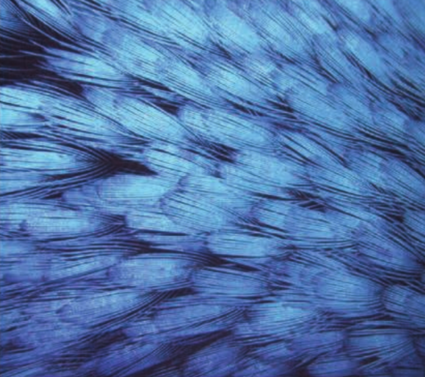
There’s a reason why the word “peacock” has become a verb synonymous with commanding attention. Of course, the size of the peacock tail is enough to turn heads, but it wouldn’t be nearly as beautiful without its signature iridescent, or angle-dependent, color. The brilliant colors of the peacock come from the interaction of light with the nanoscale structure of the feathers, which is much different from the origin of color in regular dyes and pigments. In today’s paper, Jason Forster and his colleagues in the Dufresne group developed a simple way to make colors that is inspired by the structures in certain bird feathers.
Figure 1. An iridescent peacock feather. Source: http://www.publicdomainpictures.net/pictures/100000/velka/peacock-feather.jpg
Colors come from the way our brain interprets different wavelengths of light. Most colors we encounter in dyes and paints are a result of absorption. Certain chemicals absorb specific wavelengths of light, and the other wavelengths are reflected; the colors we see are due to those reflected wavelengths. However, not all colors come from absorption. The color of the sky is perhaps the most widely seen example of this. The molecules that make up air scatter much more light at small wavelengths, which corresponds to blue light.
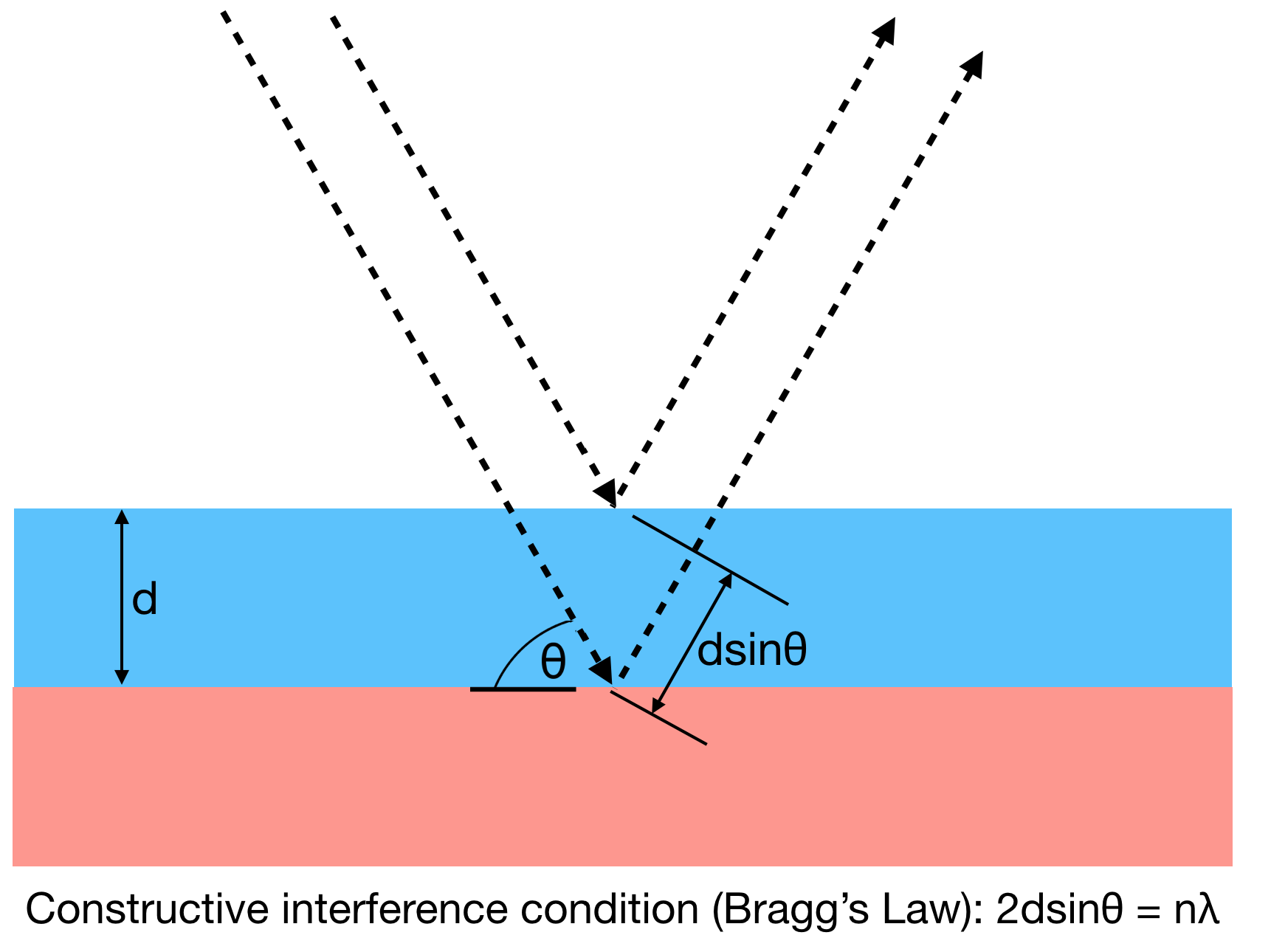
The iridescence of the colors in the peacock feather is caused by constructive interference due to the nanoscale structure of the feather. To explain this, let’s look at a simplified picture. If you have a layered stack of materials, some light will be reflected from each layer in the stack (Figure 2). Since the light reflected from the layers at the bottom stack will have traveled farther, the different sets of reflected waves will be shifted out of phase. When the waves are shifted by exactly one wavelength, they add constructively and give a stronger reflection. This constructive interference happens at a wavelength which depends on the thickness of the layers, their index of refraction, and the angle at which the light is sent and detected. Structural color is a result of the stronger reflectance at a particular wavelength due to this constructive interference of light.
Figure 2. Diagram depicting path length difference from reflection from different layers that gives rise to constructive interference.
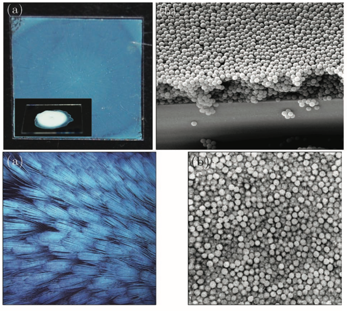
Structural color can arise in many different types of structures, from bird feathers and butterfly wings to soap bubbles and opals, but today’s paper is about a type of structural color made from plastic spherical particles. These spheres are only a few hundred nanometers in diameter, on the order of the wavelength of visible light, and they are so small that they can remain suspended in water for long periods of time, forming a colloidal suspension. Jason Forster and his colleagues in the Dufresne group made structurally colored films by starting with a small volume of a colloidal suspension of these particles and allowing it to dry, causing the particles to pack together and self-assemble into structures with color.
The way the particles packed greatly impacted the color of the film. When the researchers used spheres that were all the same size, the particles formed a crystal (an ordered arrangement made of a repeating unit cell) as the suspension dried. In a crystalline structure such as the peacock feather, the structural color is iridescent, or angle-dependent. This angle-dependence of color arises because the angle that light is sent into the sample will affect the distance it travels through the material, therefore changing the wavelength at which the light will constructively interfere. However, the researchers found that when they mixed spheres of two different sizes, the spheres could no longer form a crystal, and instead formed a disordered structure (Figure 3, top). This structure was isotropic, meaning that it looked the same from any angle. The structural color of a crystalline sample is iridescent because light travels different path lengths through it at different angles. Because the isotropic structure is essentially the same at all angles, the color is the same at all angles.
Figure 3. Top left: Photo of a structurally colored film. Top right: Scanning electron micrograph of particles in a film comparable to the one on the left. Bottom left: Photo of bird feathers of Lipodothrix Coronata. Bottom right: Tunneling electron micrograph of bird feathers on the left. Adapted from Forster et al.
By making a more disordered structure, Forster and his colleagues were able to make a more uniform color! These disordered assemblies of spheres bear a striking resemblance to the nanoscale structures found in bird feathers such as Lipodothrix Coronata (Figure 3, bottom), which are made up air spheres embedded in a disordered array inside a matrix of beta-keratin. These bird feathers have a color similar to the particle films made by the researchers: a blue color that doesn’t change with angle.
Our eyes are a useful tool for observing colors, but they are not the most precise way to measure light. If we want to compare colors precisely and quantitatively, the best way to do that is by looking at a reflectance spectrum. A reflectance spectrum tells you the amount of light reflected from an object at a range of wavelengths. You can measure a reflectance spectrum by shining light at a colored sample and using a spectrometer to detect the reflected light. Combined with a computer, a spectrometer allows you to record an intensity value for a range of wavelengths, giving you a full intensity spectrum. The reflectance spectrum is found by normalizing this data against a perfect reflector such as a mirror or a white material, giving you the percent of light reflected at each wavelength. So if you were to measure the reflectance of a blue material, you would have a spectrum with a peak in the wavelengths that correspond to blue light (~450-495 nm).
One way to infer the reflectance spectrum of a material that has no absorption is to measure transmittance. To measure the transmittance spectrum, you can move the detector to the side opposite to the incident light, so it detects the light that goes through the sample. If you were to measure the transmittance spectrum of this same blue material, you would expect to see a dip corresponding to the blue wavelengths. The blue light would not make it through to the other side because it was reflected.
The researchers measured the transmittance spectra for their structurally colored samples and found that the blue isotropic structural color and the blue crystalline structures both showed a dip in the blue wavelengths (Figure 4). However, the dip in the isotropic structure data was much broader and more shallow, meaning that less light was reflected at that wavelength, making the color less bright and saturated.
Figure 4. Transmittance spectra for isotropic and crystalline samples. The top three curves are spectra for the isotropic samples at different angles. The bottom three curves are spectra for the crystalline samples at different angles. Top inset: diagram showing sample angles. Bottom inset: scanning electron micrograph for a crystalline sample. Adapted from Forster et al.
But the quality of the color wasn’t the only thing that changed in the spectra of the isotropic structures. In these samples, the transmittance dip stayed at the same range of wavelengths even when the measurement angle changed, while the dip in the spectrum of the crystalline structure shifted as the measurement angle was changed. By eye, the researchers also saw that the disordered structures made angle-independent color, and the ordered structures made iridescent color. The measurements of the crystalline and isotropic structures show that there is a tradeoff between saturation and angle-independence in structural color.
The thickness of these isotropic structurally colored films also greatly affected the saturation of their color. Films that were just a few micrometers thick had a bright blue color, while much thicker films looked nearly white. The researchers found that adding some carbon black– black nanoparticles that absorb light at all visible wavelengths– made the colors of the thick films more vibrant (Figure 5). The carbon black works by reducing the effective thickness of the samples, absorbing light before it can travel through the entire layer of the sample and causing it to look like a thinner sample.
Figure 5: Isotropic structurally colored films with different amounts of carbon black. The concentrations of carbon black as weight percent are listed beneath the samples. Adapted from Forster et al.
This work showed that structural color, both iridescent and angle-independent, can be made using simple methods that could potentially make the colors in large volumes for real-world applications. Because these colors come from structure and not absorption, they will not fade over time as current dyes do. In addition, one material can be used to make a range of different colors by tuning the structure, so these assemblies could be used as colorimetric sensors that change color in response to environmental changes such as strain or temperature.