active matter – Page 2

2018-05-302018-05-31

Mob mentality improves animal sensing

Original paper: Emergent Sensing of Complex Environments by Mobile Animal Groups

Imagine you forget to bring money for lunch, and you overhear a teacher mention that there is free pizza somewhere on the third floor of your school. If you’re alone, you might walk around the third floor, trying to detect signs of pizza – does a room smell delicious? Do you see a suspicious stack of pizza boxes by the door to the gym? Just by using your senses, you can find the pizza. However, it is likely that there are other students on the third floor who also want free food. Maybe if you follow a crowd of students all walking in the same direction and talking about whether they want a Hawaiian or pepperoni slice, they might lead you directly to the pizza!

Which of these methods will be more effective? Following environmental signals, such as the smell of cheese, or social signals, such as the people all heading in the direction of potential pizza? In “Emergent Sensing of Complex Environments by Mobile Animal Groups,” Andrew Berdahl and colleagues seek to find out how searching in groups enhances the sensing ability of animals.

The researchers used a fish called the golden shiner to study this kind of mob mentality. These fish live in large schools in shallow water and prefer darker habitats. Fish school together for many reasons. For example, it helps them avoid predators and gain advantages in hunting. In this experiment, the researchers asked whether schooling helps the fish find their preferred darker spots in the water. A school of golden shiners searching for dark spots in water is a convenient model system, but the researchers stressed that the results from this study can be applied to any group of organisms looking for any environmental cue.

Berdahl and his colleagues set up a large, shallow tank for fish to swim in. The tank was in a dark room, and a projector was used to impose light patterns on it. The patterns consisted of a bright tank (similar to an overcast day) with dark patches (similar to twilight). The dark patches moved around randomly at a constant speed, with the fish expected to follow the patches.

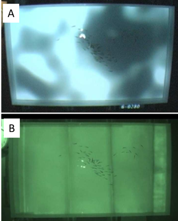
Fish were tested as individuals and as groups from 2 to 256 fish. To track the fish in both light and dark regions, the researchers used infrared (IR) light that the fish can’t see and took videos of the fish with an IR camera. The fish could then be tracked using image analysis. You can see the visible light and IR images of the fish in a dark spot in Figure 1.

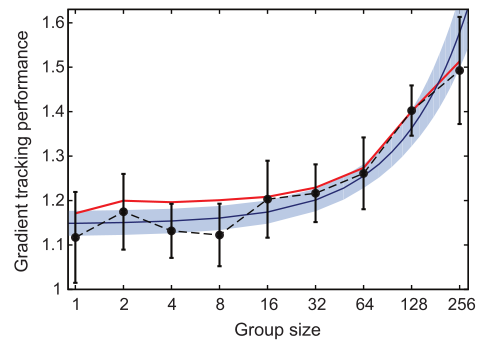
How well the fish stayed in the dark was measured with a performance metric, $latex \Psi$ (psi). This number measures how good the fish are at staying in the dark. Specifically, it measures the average inverse of brightness at all the fish positions averaged over time [1]. If $latex \Psi = 1$, the fish did not try to stay in the dark at all; the performance was better as $latex \Psi$ increased. The data in Figure 2 shows that $latex \Psi$ increases with group size – bigger groups make the fish better at tracking dark patches.

Figure 2: Ability of fish to track the dark patches in the tank improves with group size. Points with error bars represent the averages over all the experiments at each group size, and the blue line is the statistical fit. The red line is the results from simulations implementing the rules of the collective behavior of the fish. Image adapted from Berdahl and colleagues’ original paper.

The researchers wanted to find out whether the fish were responding to the changes in the environment or the behavior of their neighbors. They calculated a social vector and an environmental vector for each fish. The social vector measures what direction a fish’s closest neighbors are. If all of the fish’s neighbors are to its left, there will be a strong social vector to the left; if the neighbors are all spread out around it the social vector will be very small [2]. The environmental vector points in the direction of the darkest position near the fish[3]. The researchers calculated how correlated each vector was with the acceleration of the fish. When the magnitude of the social vector was very high – a fish’s neighbors were all located in the same direction from it – the fish listened to the social vector and swam to where their neighbors were. They did not respond as strongly to what direction the nearest dark patch was in. In other words, fish respond much more to nearby clusters of neighboring fish than to their environment, similarly to how you might pay attention to your friends in your hunt for pizza rather than smelling around.

Although fish did not respond to the changes in the lighting of the tank directly, as measured by the environmental vector, they did respond to the environment: fish swam faster in lighter regions, and slower in darker ones. They responded to the scalar brightness at their position in the tank, rather than how much the brightness was changing. If a mountain climber behaved like these fish, he would climb more slowly at higher altitudes (responding to the elevation) but not change his speed based on the steepness of the slope (not responding to the gradient in elevation).

These two main behaviors of the fish, swimming towards their neighbors and changing their speed based on the lighting, made group tracking of dark patches very effective. The researchers highlight two examples of how this could work. The first example is that of fish traveling next to a dark patch. Some of the fish are located on the brighter side of the dark patch and swim faster. Other fish are in the darker region and swim slower. This causes the whole group to turn towards the slower fish and therefore into the dark patch. The second example is of a group of fish traveling into a dark patch. As fish enter the dark patch, they slow down. The rest of the group follows them and slows down as well. This increases the number of fish in darker regions.

The researchers created a computer model that simulated behaviors of fish with these two rules: following their neighbors and changing the speed according to the brightness of the light at their positions. Although they did not build in any explicit response to the changing light gradient, the groups of simulated fish responded the same as the real fish in the experiment, as seen in Figure 2. Berdahl and his colleagues conclude that the response of the fish to the environment arose simply from those two rules, and the ability of groups to track dark patches increased with larger numbers of fish.

The researchers emphasize many times that the results of this study are applicable to any group sensing any field, not just fish in a light field. The results could apply to bacteria seeking food, or robots seeking a resource to collect. If, for some reason, a group of animals is broken up – for example, there are fewer fish in a school due to overfishing – the remainder of the fish in the school might not be as well equipped to seek out darker patches to hide from predators. This study highlights the importance of paying attention to your neighbors and the advantages all living organisms gain from working in groups – like helping a hungry student find some pizza!

[1] The performance metric is defined as:
$latex \Psi=\frac{\langle \langle 1-L \rangle_{fish}\rangle}{\psi_{null}}$
where L represents the light level and $latex \psi_{null}$ normalizes $latex \Psi$ so that $latex \Psi = 1$ implies that fish do not track the light at all. The inner angle brackets represent the average of the darkness, $latex 1- L$, taken over all fish, and the outer angle brackets represent the average taken over all time

[2] The social vector is defined for each fish as:
$latex S_i=\sum \frac{c_j-c_i}{|c_j-c_i|}$
where ci represents the position of the ith fish, so cj–ci is the difference between the positions of the ith fish and its neighbor, the jth fish. It is normalized by the magnitude of that distance. The sum is taken over all the fish within seven body lengths of the ith fish, for each fish

[3]The environmental vector is the negative of the gradient of the light field for each fish, i:
$latex G_i = -\nabla L\mid_i$

2018-01-242018-04-14

How swimming bacteria spin fluid

Original paper: Fluid Dynamics of Bacterial Turbulence

The next time you’re washing your hands, start by turning the water on just a little. Notice how clear is the flow of the water from the tap. There aren’t any bubbles in the water, and when you put your finger in the stream, it smoothly flows around it. This is called laminar flow. Now keep increasing the water flow until it is very fast and rough. The chaotic nature of the flow in this stream is called turbulence, and how a flow turns from being laminar to turbulent is a popular area of research. In general, turbulent flows are very fast and are made from fluids that are not very thick.

In today’s study, Dunkel and his colleagues investigate how bacteria can make flow patterns that look turbulent – chaotic and full of vortices – even though bacteria are tiny and slow. The bacteria push the fluid around as they swim and create vortices, spinning regions in the fluid. The 5 ?m long bacteria create vortices with diameters of 80 ?m by swimming at the speed of 30 ?m/s!

To determine whether a fluid flow is turbulent or laminar, the Reynolds number, a ratio of the strength of the flow (inertial forces) to how much the fluid resists motion (viscous forces) is used and defined as [1]:

$latex Re = \frac{\rho V D}{\mu}$

It depends on the fluid density ?, flow speed V, the length of an object D (for example, the diameter of a bacterium), and flow viscosity, or thickness, ?. When the Reynolds number of a flow is high, the inertia of the fluid (how powerfully it flows), is much higher than its viscosity (how thick the fluid is). In this case, the resistance of the fluid to small fluctuations in its motion is not enough to prevent the fluctuations from growing and spreading. Before you know it, your previously smooth, easily predictable flow is chaotic and full of vortices – it has transitioned to turbulence.

Typically, flow in a pipe like that in a tap becomes turbulent at a Reynolds number of 2300; the flow of air over an airplane begins transitioning when the Reynolds number is about a million. Bacteria are so tiny and slow that their Reynolds number is very small – on the order of $latex 10^{-5}$.

The researchers in this study investigate turbulent-like fluid behavior caused by swimming bacteria, B. Subtilis, in a fluid. B. Subtilis is a rod-like bacteria that swims by pushing its surrounding fluid with its flagellum (or tail). The researchers grew the bacteria in a nutritious fluid medium, and they added small, 1 micrometer beads to the fluid to act as tracer particles. When tracer particles are added to a fluid, you can see them being pushed around by its flow. If the particles are small enough, tracking them can be used to show how the fluid is moving. Thus, the experiment consisted of a suspension (a mixture in which particles do not dissolve) of bacteria and particles in the fluid.

The researchers loaded this suspension into sealed microfluidic cylindrical chambers with a 750 ?m radius and 80 ?m height (Figure 1). Since the chamber was sealed, the bacteria grew tired and did not move as much as they ran out of oxygen, so their activity levels decreased during the 10 minutes they spent in the chamber. Thus, by waiting several minutes between sets of measurements, the researchers were able to test how the bacteria affected the fluid at different energy levels.

The researchers took high-speed 2D videos of slices of the suspension containing the bacteria and the particles in the middle of the cylinder (even though the motion of the bacteria was in 3D). They used visible light to illuminate the motion of the bacteria and fluorescent light to view the motion of the tracer particles through a microscope.

setup — Figure 1: Bacteria and tracer particles in the field of view of the camera. Although the entire test chamber is filled with fluid, only the 2D cross-section in the center of the cylinder is in focus.

The researchers used two methods to measure the motion of the suspension of bacteria and particles. First, by monitoring the motion of the bacteria, they obtained vectors showing how the bacteria were moving. Trajectories of bacterial movement were calculated by comparing the position pattern of the bacteria from one image frame to another. In the second approach, they tracked the motion of the particles in the flow by comparing the actual position of the particles from one image frame to the next. The researchers used both methods (monitoring patterns of bacterial motion and tracking individual particle positions) to make sure the flow fields measured from bacteria were an accurate representation of the flow. Since the tracer particles used by the researchers were very small, with diameters of 1 micrometer, they were small enough to be reliably pushed by the flow.

The typical results the researchers got are shown in Figure 2, with visible vortices.

The researchers measured the velocity distributions of the bacteria. They found that the results from the tracer particles and the bacteria had the same distributions – the flow of the bacteria and solvent were very similar, and the flow of the bacteria could be used to represent the fluid flow. However, it is possible that the particles were pushed around by the bacteria, and not by the motion of the fluid itself, which is not mentioned in the paper.

To analyze the average motion of the bacteria, the researchers calculated various properties of the velocity field. They calculated the vorticity, $latex \omega_z$, or how much the bacteria rotated the fluid. The average of the square of the vorticity throughout the 2D experimental plane is called the enstrophy, $latex \Omega_z$. They then calculated the kinetic energy of the flow, $latex E_{xy}$, the energy a fluid has because of its speed, and also calculated its average throughout the space (1). Although the instantaneous kinetic energy and vorticity fluctuated as the bacteria moved, the average kinetic energy and enstrophy over time were approximately constant throughout the 50 seconds of recording.

The researchers then measured two properties of the flow with functions called the VCF (“equal-time spatial velocity autocorrelation function”) and the VACF (“two-time velocity auto-correlation function”). The first function, the VCF, measures how the velocity of the fluid changes throughout the space (the 2D slice of the cylinder). If this function goes from positive, velocities in the same direction, to negative, velocities in different directions, then it indicates that there is a vortex in the fluid (Figure 3a). The results of the VCF are shown in Figure 3b. The researchers calculated that the radius of a vortex in the fluid was $latex R_v = 40 \mathrm{\mu m}$ from the VCF. The vortex radius did not change with the kinetic energy of the flow.

The average enstrophy was found to be linearly proportional to the time-averaged kinetic energy by about half the vortex radius ($latex \Lambda = \mathrm{24 \mu m}$) over all the energy scales tested:

$latex \overline{\Omega_z} =\frac{\overline{E_{xy}}}{\Lambda^2}$

So when bacteria have more energy, the fluid has a higher tendency to form vortices and rotate (but the vortices will be the same size).

The second property the researchers calculated was the “VACF”. The VACF measures how the velocity changes over time. The VACF represents the memory of the fluid. If it decays to 0 slowly, that means the velocities stay similar for a long time; if it decays quickly, the velocity changes in a very short time. The results of the VACF are shown in Figure 3c. The researchers found that at higher energies, the system has a shorter “memory”. The VACF shown in black has the highest energy, and decays much faster than the VACF shown in purple, which has the lowest energy. In bacterial turbulence, bacteria add energy to the system by swimming to make small vortices, which then lead to larger vortices. This is the opposite of how vortices form in a non-active turbulent fluid, where the energy is added to the larger vortices that create smaller vortices because of the fluid’s viscosity.

correlation — Figure 3. (a) Diagram of a vortex. The blue and green vectors are correlated (positive VCF), showing that there is no vortex between them; the blue and red vectors are anticorrelated (negative VCF), showing the presence of a vortex. VCF (b) and VACF (c) of the bacterial motion. The minimum value of the VCF indicates a vortex with a 40-micron radius. The VACF varies with energy when plotted as a function of the time lag. Inset: energy as a function of time; the black spheres show the highest energy and data in purple is at the lowest. Figure modified from the original paper.

Finally, the researchers present a recently developed theory for the flow caused by bacteria. This theory is a continuum model equation – it treats the suspension of fluid, bacteria, and particles as if it were a continuous material, and accounts for the effects of the fluid flow and the forces the bacteria apply to the system.

The equation in the theory can be modeled to predict how the suspension will move. If the parameters of the equation in this theory are chosen to represent flow without bacteria, it simplifies to a theoretical fluid flow model. The researchers chose coefficients in the equation known to represent bacteria that push the fluid, like B. Subtilis in this experiment. They found that the model was accurate to within 10%-15%, making it a good candidate for a quantitative description of bacterial turbulence.

In today’s paper, Dunkel and his colleagues made significant contributions to the understanding of bacterial turbulence. The researchers developed a method to show that the motion of the bacteria swimming in a fluid can be used to measure the motion of the fluid itself. They developed a mathematical model of the motion and tested it with their experimental results to create a method for quantitatively studying how bacterial motion affects fluid flows. The observations they made can be used to compare bacterial turbulence to traditional turbulence in fluid mechanics, and give insight into how other fluids with active particles might behave.

[1] Fox, Robert W., Alan T. McDonald, and Philip J. Pritchard. Chapter 2, Introduction to fluid mechanics. Vol. 5., New York: John Wiley & Sons, 1998.

[2] Dunkel, Jörn, et al. “Fluid dynamics of bacterial turbulence.” Physical review letters 110.22 (2013): 228102.

(1) The vorticity, $latex \omega_z$, is calculated by taking the difference between the change in the y-component of the velocity, $latex v_y$, in the x-direction and the x-component of the velocity, $latex v_x$ in the y-direction:

$latex \omega_z = \frac{\partial v_y}{\partial x} – \frac{\partial v_x}{\partial y}$

The average kinetic energy (represented by angle brackets is calculated as:

$latex E_{xy} = \frac{v_x^2+v_y^2}{2}$

As the mass of the bacteria was constant, the energy depends only on the measured velocities of bacteria, and mass was not included in the calculation. As you may remember, a range of energies was tested by varying the bacterial activity.

The enstrophy, $latex \Omega_z$, is calculated as the average of the vorticity as:

$latex \Omega_z = \langle\frac{\omega_z^2}{2}\rangle$

2017-10-272018-04-14

Fluids That Flow Themselves

Original paper: Transition from turbulent to coherent flows in confined three-dimensional active fluids (Non-paywall version here.)

Disclosure: The first author of the paper discussed in this post, Kun-Ta Wu, did his Ph.D. at New York University, in the same research group as the present writer (CPK). At NYU, both Wu and CPK worked on topics unrelated to the research discussed here.

*****

When we think about fluid flow, we generally think of motion in response to some external force: rivers run downhill because of gravity, while soda moves through a straw because of the pressure difference created by sucking on one end. Recently, however, scientists have become interested in a class of fluids that have the capacity to move all by themselves — the so-called “active fluids.” Active materials — of which active fluids are a subset — are distinct from regular materials because energy is injected into the system at the level of individual molecules. In today’s paper, Kun-Ta Wu and his co-workers explore how such a material can turn its stored chemical energy into useful work: cargo transport.

Why are active materials so interesting? For one thing, many biological systems are active — for example the actin filaments that drive muscle contraction or bacterial swarms. Although active systems are both common and important in our everyday lives, the physical laws that govern their behavior are not well understood [1]. Studying artificial active systems, which are much simpler than living ones, might give us insight into this difficult problem.

As well as helping us to understand basic physics and biology, Wu and his co-workers hope that their research will move us closer to producing artificial materials that transport cargo without adding energy from an external source — a self–powered fluidic conveyer belt [2]. Such a material would be totally different from those that we currently use, and would greatly expand the possibilities available to engineers in fields such as microfluidics and soft robotics.

Wu’s research focuses on a system made up of protein molecules that assemble into cylindrical rods called microtubules. While microtubules are very important in biology [3], Wu uses these tiny rods, suspended in water, to make an artificial active fluid. As well as microtubules, Wu adds two other critical ingredients: kinesin molecular motors, and ATP (adenosine triphosphate), a chemical that many biological systems use as an energy source [4].

fig1 — A sliding force is generated between microtubules by the action of molecular motors. (Adapted from Figure 1 of the original paper.)

A single kinesin molecule attaches to two parallel microtubules and creates a lateral force that slides or “walks” them along each other. A single “step” of this walk involves a chemical reaction that converts one ATP molecule into ADP (adenosine diphosphate), a lower-energy state, thereby converting chemical potential energy into motion. A collection of millions or billions of microtubules (and a similar number of kinesin and ATP molecules) forms a material that writhes and squirms without any forces acting upon it. In the following video, Wu records the motion of both the microtubules themselves (they’re tagged with a fluorescent red dye), and micrometer-sized green particles, which he uses to trace the flow.

Video 1 Using fluorescence microscopy, Wu and colleagues can observe the motion of microtubules (red), as well as test cargo — colloidal particles (green) that are carried along in the flow generated by the motion of microtubules. (Movie 1 of the original paper.)

.
But converting energy into useful work doesn’t just require motion; it requires motion that is controlled, directed, and uniform over time — coherent motion. This brings us to the main finding of Wu and coworkers: in the microtubules-motors-ATP system, coherent motion can be produced by controlling the shape of the container. Placed in a large rectangular box, the flow in the middle of the box (“in the bulk”) is turbulent but directionless (see panel A of the below figure). However, when placed in a ring with appropriate dimensions, the flow spontaneously organizes into large-scale circular patterns that are capable of transporting cargo — like fluorescent colloidal particles — over lengths of centimeters or even longer (panel B below).

fig2 — Panel A shows the pattern of flow of a bulk sample of active fluid. The arrows represent the velocity field, and colors represent the normalized *vorticity* of the flow: the extent to which it is rotating clockwise or anticlockwise in a local frame of reference. The left half of the panel shows a snapshot of the flow at a single instant in time, while the right half shows the time average. (This convention is also used in the other flow visualizations shown in this post.) In the time-averaged plot, both velocity and vorticity are almost zero: the flow is turbulent but directionless. Panel B-i shows the ring geometry of one of the sample chambers Wu uses to create coherent flow, and B-ii shows the flow pattern in that chamber. Unlike in the bulk sample, a long-lived circular pattern is generated that pushes the cargo around the ring. (Adapted from Figure 1 of the original paper.)

Interestingly, whether or not this happens is controlled only by the aspect ratio of the container: the channel width divided by its height [5]. Coherent flow is observed when the aspect ratio is between ? and 3; in other words, it disappears if the ring is too flat or too tall. Additionally, Wu shows that the direction of the flow– whether it goes clockwise or counterclockwise — can be controlled by decorating the outside of the container with appropriately shaped notches, which Wu calls ratchets.

Finally, the researchers show that the appearance of directed flow coincides with the onset of nematic order: in circulating samples, the rod-like microtubules tend to align with their neighbors, while in the turbulent samples, they are oriented randomly. According to Wu, this alignment allows the fluid to collectively push itself off the walls of the container, thus generating global circulation.

fig3 — Wu and co-workers use ratchets — small asymmetrical notches on the outside of the ring — to control whether the flow is clockwise (CW) or counterclockwise (CCW). The scale bar shows that flow is coherent over lengths of centimeters. (Adapted from Figure 3 of the original paper.)

Of course, this paper only scratches the surface of the technological potential of active materials. Research on this, and similar ideas, continues both at Brandeis University, where this research was done, and in Worcester Polytechnical Institute, where Wu has recently been appointed professor. Here, according to his website, Wu aims to “advance our understanding of self-organization of active matter as well as to create unprecedented bio-inspired materials.”

*****

[1] Physical systems at thermodynamic equilibrium obey the Boltzmann distribution — a formula that (in principle) allows us to calculate macroscopic properties of many-body systems, if we know the interactions between the constituent particles. We don’t know of a similar theory that describes the behavior of out-of-equilibrium systems, and active systems are by definition out of equilibrium.

[2] Of course, the energy ultimately has to come from somewhere. In the case of the material studied by Wu et al, the conveyer belt would have to be “charged” with fresh ATP before use.

[3] In particular, microtubules are the most important structural component of the mitotic spindle – the sub-cellular structure that pulls chromosomes copies apart during cell division.

[4] Wu also adds a chemical known as a depletant, which makes the microtubules bundle together, allowing the kinesin to slide them along each other.

[5] Wu also studies cylinders and shows that a similar geometrical parameter controls the appearance of coherent flow.