Look inside a glass of milk. Still, smooth, and white. Now put a drop of that milk under a microscope. See? It’s not so smooth anymore. Fat globules and proteins dance around in random paths surrounded by water. Their dance—a type of movement called Brownian motion—is caused by collisions with water molecules that move around due to the thermal energy. This mixture of dancing particles in water is called a colloid.
Colloids are one of the classic topics in soft matter, a field of physics that covers a broad range of systems including polymers, emulsions, droplets, biomaterials, liquid crystals, gels, foams, and granular materials. And while I can keep adding items to this list, I can’t give you a precise definition for soft matter. I’ve never seen a completely satisfying definition, and I’m not going to even attempt to provide that here. But I can give you a taste of some of the definitions, and I hope you’ll come away with the feeling that you sort of know what soft matter is.
The phrase “soft matter” brings to mind pillows and marshmallows. These things fall under physicist Tom Lubensky’s definition (given in a 1997 paper) of soft materials as “materials that will not hurt your hand if you hit them.” And while many materials in soft matter are too squishy to hurt you, some of them might—cross-linked polymers can be pretty hard. And what about colloids? Slapping milk won’t hurt, but it also seems strange to call milk soft.
To understand what the “soft” refers to in “soft matter”, we first have to know where the name came from. The French term “matière molle” was coined in Orsay around 1970 by physicist Madeleine Veyssié, who worked in the research group of one of the founding fathers of soft matter, Pierre-Gilles de Gennes. The phrase apparently started as a private joke within the de Gennes group (don’t ask me what it meant), and the English translation of “soft matter” was popularized by de Gennes in a lecture he gave after winning the Nobel prize in 1991. De Gennes wrote that soft matter systems have “large response functions”, meaning that they undergo a large (don’t ask me how large) change in response to some outside force. So it seems we’re meant to take “soft” to mean something closer to “sensitive”, not necessarily soft in a tactile sense.
Now we can think about why colloids are soft from a different perspective. Remember that milk droplet under the microscope? The fats and proteins move around in the droplet due to thermal energy in the water; they are “sensitive” to the forces caused by thermal energy.
But even this “large response functions” idea doesn’t describe everything in soft matter. Some topics often considered a part of the field are concerned with general mathematical concepts instead of particular materials or systems. Take, for example, particle packing—the way particles arrange themselves to fit into confined spaces. Studying how particles can be arranged to pack on a curved surface is a mathematical problem and isn’t directly related to large response functions. However, since classic soft matter systems such as colloids are made up of particles you might want to pack, it makes sense to include packing as part of the field.
For every definition you give for soft matter, you can find a system that doesn’t quite fit. In an APS news article from 2015, Jesse Silverberg described soft matter as “…an amalgamation of methods and concepts” from “physics, chemistry, engineering, biology, materials, and mathematics departments. The problems that soft matter…examines are the interdisciplinary offspring that emerge from these otherwise distinct fields.” So maybe it’s not that important to have a rigid definition for soft matter; maybe its indefinability should be part of its definition. Soft matter is a field where the lines between traditional scientific disciplines are becoming ever more blurred—or, rather, soft.
Physics is a discipline that attempts to develop a unifying, mathematical framework for understanding diverse phenomena. It connects things as different as planets orbiting the sun and a ball thrown through the air by showing that both these motions come from a single equation [1]. Living things do not seem to obey such simplicity, but hidden beneath all the diversity and complexity of life are remarkably universal patterns called scaling laws. In a landmark 1997 paper by Geoffrey West, James Brown, and Brian Enquist, a simple explanation is given for how all organisms, from fleas to whales to trees, can be thought of as non-linearly scaled versions of each other.
A scaling law tells you how a property of an object, say the rate at which energy is consumed by an organism (its metabolic rate), changes with the object’s size. Just by looking at the data, many quantities scale as a power law of the mass,
$latex A \propto M^{\alpha}$ (Eq. 1)
where ? is some number that, from the data, always seems to be a multiple of 1/4 [2]. West, Brown, and Enquist build a theory showing how biology could have come up with this 1/4 power law, but in this article, I’m just going to focus on one specific example. I’m going to walk through the author’s arguments for how the metabolic rate, the rate at which an organism consumes energy, scales with an exponent of 3/4. They show that it all comes up from some basic assumptions about the networks that distribute nutrients to your body — your circulatory system [3].
These networks are assumed to have two characteristics [4]. First, they are space-filling fractals. Fractals are shapes made of smaller, repeating versions of themselves no matter how far you zoom into it. However, our fractal blood vessels can’t get arbitrarily small, they have a “terminal unit”— the capillary. The second assumption about these networks is that all terminal units are the same size, regardless of organism size. With these two assumptions, the authors are able to derive the 3/4 power law for metabolic rate.
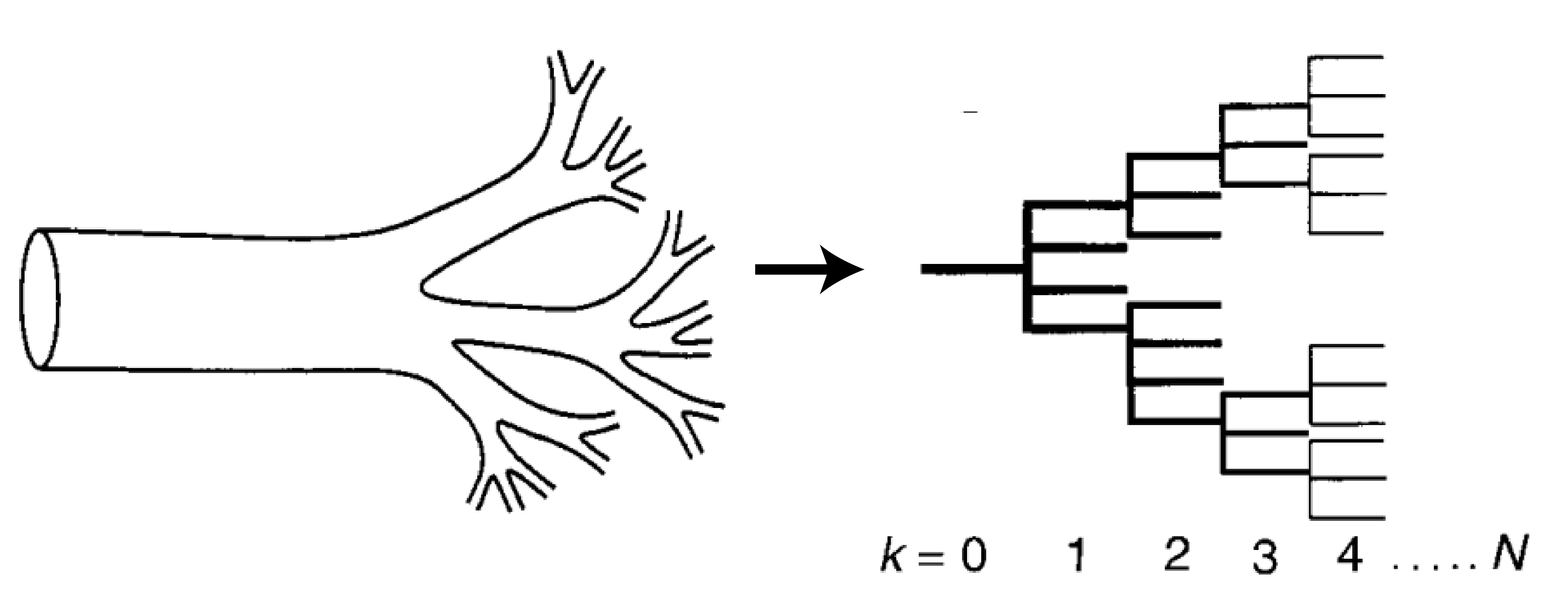
Figure 1: Cartoon of a mammalian circulatory system on the left, which can be represented as a branching network model on the right. Adapted from Figure 1 of the original paper.
First, let’s build up a picture of what these networks look like. Figure 1 shows how the circulatory system can be thought of as a network structured into N levels, where each level k has $latex N_k$ tubes. At each level, a tube breaks into a number ($latex m_k$) of smaller tubes. Each one of these tubes is idealized as a perfect cylinder with length $latex l_k$ and radius $latex r_k$, as shown in Figure 2.
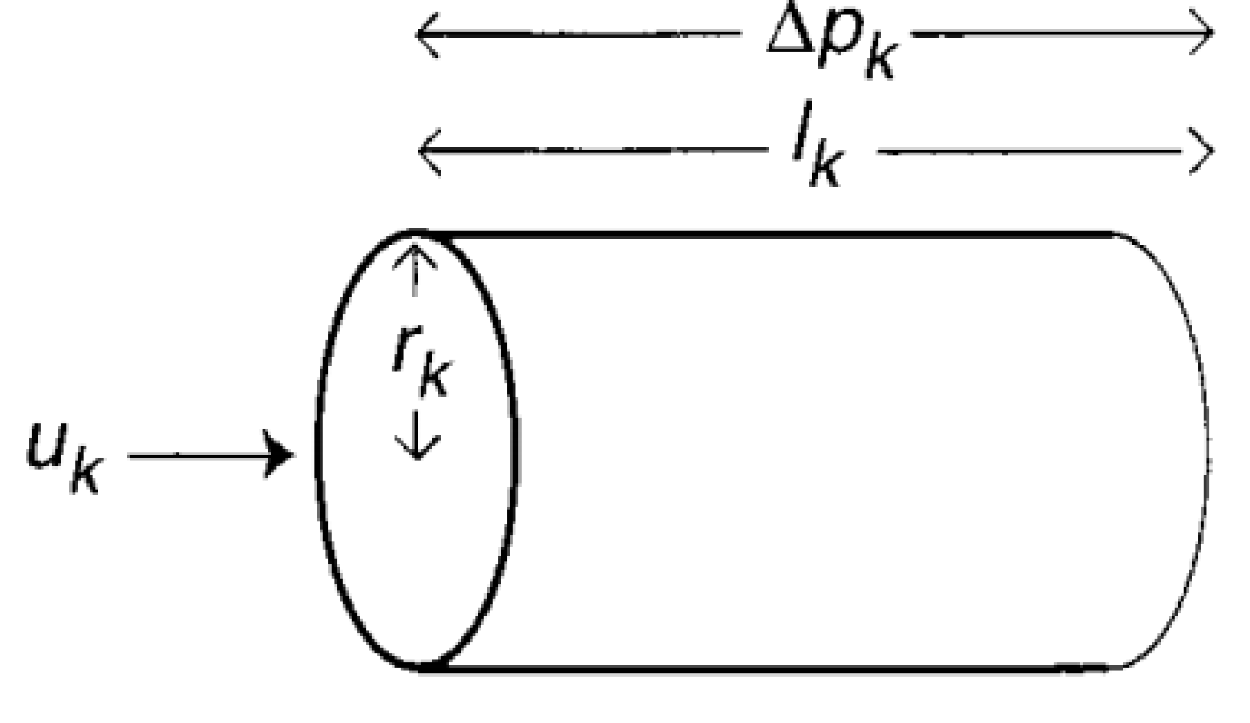
Figure 2: Illustration of the different parameters that each tube on the kth level of the network has. Adapted from Figure 1 of the original paper
How does blood move through this network? Well, the blood flow rate at each level of the network must be equal to the blood flow rate at every other level. Otherwise, you would have the equivalent of traffic jams in your arteries. You don’t want those. If the blood flow speed through one tube in the kth level is $latex u_k$, the blood flow rate through the entire kthlevel is
Your metabolic rate, B, depends on the flow rate through your capillaries, $latex \dot{Q}_{cap}$, so the authors assume that the two are proportional to each other: $latex B \propto \dot{Q}_{cap}$. Because all terminal units are the same size, the only variable left in Eq. 2 to relate to an animal’s mass is $latex N_{cap}$.Assuming that B scales like $latex B \propto M^{\alpha}$, and the authors predict
$latex N_{cap} \propto M^{\alpha}$ (Eq. 3)
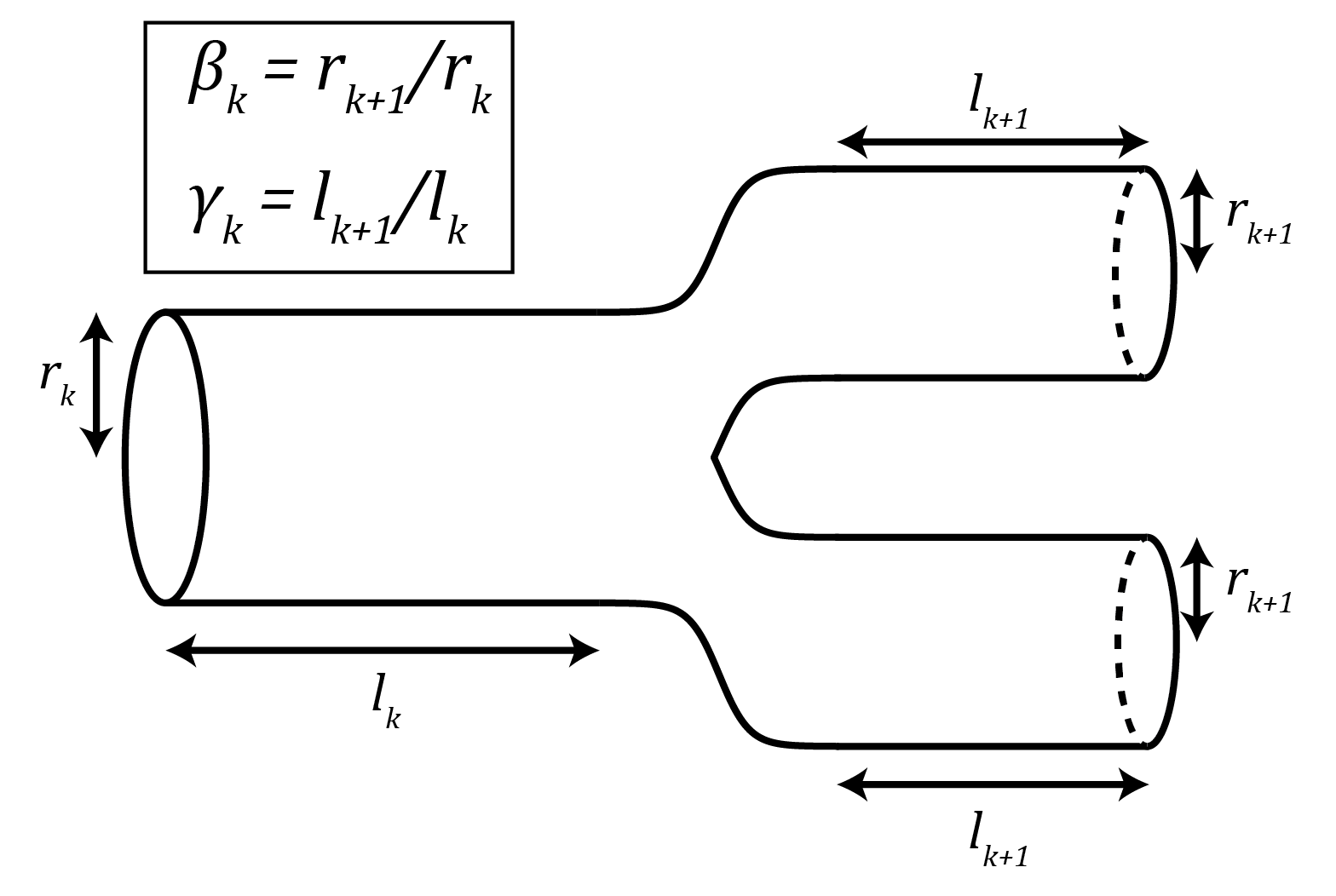
Figure 3: Schematic of a branching point along the network, illustrating the definitions of the ratios $latex \beta_k$ and $latex \gamma_k$. In this case, $latex m_k = 2$.
To figure out the value of the exponent $latex \alpha$, the key is to get $latex N_{cap}$,which depends on the size of the organism, in terms of the capillary dimensions $latex r_c$ and $latex l_c$, which do not. To do this, the authors use relations derived using the self-similar geometry of the fractal network. When a tube breaks into smaller tubes, it does so with a ratio between the successive radii, $latex \beta_k = r_{k+1} / r_k$, and another ratio between the successive lengths, $latex \gamma_k = l_{k+1}/l_k$. This is illustrated in Figure 3. Because the network is fractal, the number of tubes each branch breaks into, $latex m_k$, the ratio of radii, $latex \beta_k$, and the ratio of lengths, $latex \gamma_k$, are all assumed to be constant for every k,
Since, at every level, each branch breaks into m smaller branches, the total number of capillaries (i.e. the number of branches at level N) is $latex m^N$. Plugging this into Eq. 3,
Where $latex M_0^{\alpha}$ is the proportionality constant between $latex N_{cap}$and $latex M^{\alpha}$. Remember, we’re trying to show that $latex \alpha = 3/4$.
Now that $latex N_{cap}$ has been rewritten in terms of network properties, the authors next turn their attention to another quantity that scales with the organism size — its mass, M. To do this, the authors use the empirical fact that the total volume of blood, $latex V_b$, is proportional to the total mass of the organism, $latex V_b \propto M$. The total volume of blood is given by:
In the above equation, the first proportionality sign (summing the series) requires a calculation that’s given here. The main idea of this calculation is that, because the ratios $latex r_{k+1} / r_k$ and $latex l_{k+1}/l_k$ are each constant, the sum in Eq. 5 can be turned into a geometric series which can be summed analytically. Plugging the final proportionality from Eq. 5 into Eq. 4,
To make further progress, we have to know something about $latex \gamma$ and $latex \beta$. Every tube of the network gives nutrients to a group of cells. As every good physicist does, the authors will assume that this group of cells has the volume of a sphere with a diameter equal to the length of the tube. The volumes serviced by each successive level are approximately equal to each other, $latex 4/3 \pi (l_{k+1} / 2)^3 N_{k+1} \approx 4/3 \pi (l_k / 2)^3 N_k$. From this, they get an expression for $latex \gamma$:
Now the authors move on to $latex \beta$. Earlier, I argued that the flow rate has to be the same from one level of the network to the next to avoid “traffic jams” of blood. Since the tubes are assumed to be perfect cylinders, this boils down to the idea that the cross-sectional area of a parent tube being equal to the total cross-sectional area of its daughter tubes, $latex \pi r_k^2 = \pi r_{k+1}^2 m$. From this, the authors find an expression for $latex \beta$:
What West and his colleagues have done is use the fact that all organisms have to deliver nutrients to their individual parts to derive a general, universal scaling law. The authors go on to show that when you add a pump to the system, such as our heart, the analysis may get more complicated, but the ultimate result remains unchanged. All living things, regardless of size, seem to have arrived at the same solution for nutrient supply, building systems that are space-filling, fractal, and have the same size “terminal units”. Turns out we’re not so different after all.
$latex \alpha = 3/4$ for cross section area of aortas of mammals, tree trunk sizes
$latex \alpha = -1/4$ for cellular metabolic rate, heartbeat rate, population growth
$latex \alpha = 1/4$ for time of blood circulation, life span, embryonic growth rate ^
[3] All the arguments hold for other distribution systems, such as our pulmonary system, plant vascular systems, and insect respiratory systems. ^
[4] There’s an additional assumption that the network is designed to minimize energy, but that won’t come into play in the part of the author’s arguments that I will be presenting here. ^
There are many things that we “know” about the world around us. We know that the Earth revolves around the Sun, that gravity makes things fall downward, and that the apparently empty space around us is actually filled with the air that we breathe. We take for granted that these things are true. But how often do we consider whether we have seen evidence that supports these truths instead of trusting our sources of scientific knowledge?
Students in school are taught from an early age that matter is made of atoms and molecules. However, it wasn’t so long ago that this was a controversial belief. In the early 20th century, many scientists thought that atoms and molecules were just fictitious objects. It was only through the theoretical work of Einstein [1] and its experimental confirmation by Perrin [2] in the first decade of the 20th century that the question of the existence of atoms and molecules was put to rest. Today’s paper by Newburgh, Peidle, and Rueckner at Harvard University revisits these momentous developments with a holistic viewpoint that only hindsight can provide. In addition to re-examining Einstein’s theoretical analysis, the researchers also repeat Perrin’s experiments and demonstrate what an impressive feat his measurement was at that time.
In the mid-1800s, the botanist Robert Brown observed that small particles suspended in a liquid bounce around despite being inanimate objects. In an effort to explain this motion, Einstein started his 1905 paper on the motion of particles in a liquid with the assumption that liquids are, in fact, made of molecules. According to his theory, the molecules would move around at a speed determined by the temperature of the liquid: the warmer the liquid, the faster the molecules would move. And if a larger particle were suspended in the liquid, it would be bounced around by the molecules in the liquid.
Einstein knew that a particle moving through a liquid should feel the drag. Anyone who has been in a swimming pool has probably felt this; it is much harder to move through water than through air. The drag should increase with the viscosity, or thickness, of the fluid. Again, this makes sense: it is harder to move something through honey than through water. It is also harder to move a large object through a liquid than a small object, so the drag should increase with the size of the particle.
Assuming that Brownian motion was caused by collisions with molecules, and balancing it with the drag force, Einstein determined an expression for the mean square displacement of a particle suspended in a liquid. This relationship indicates how far a particle moves, on average, from its starting point in a given amount of time. He concluded that it should be given by
where R is the gas constant, T is the temperature, $latex \eta$ is the viscosity of the liquid, $latex N_A$ is Avogadro’s number [3], r is the radius of the suspended particle, and $latex \tau$ is the time between measurements [4]. With this result, Einstein did not claim to have proven that the molecular theory was correct. Instead, he concluded that if someone could experimentally confirm this relationship, it would be a strong argument in favor of the atomistic viewpoint.
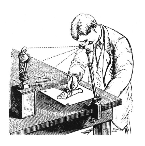
Figure 1: A camera lucida is an optical device allows an observer to simultaneously see an image and drawing surface and is therefore used as a drawing aid. (Source: an illustration from the Scientific American Supplement, January 11, 1879)
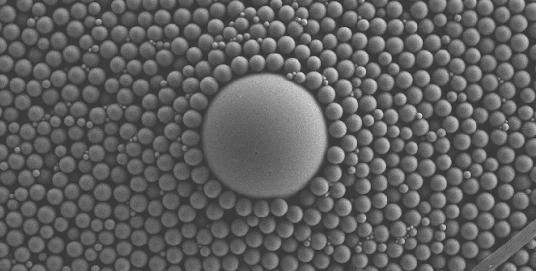
This is where Perrin came in. Nearly five years after Einstein’s paper was published, he successfully measured Avogadro’s number using Einstein’s equation, confirming both the relationship and the molecular theory behind it. However, with the resources available at the time, this experiment was a challenge. Perrin had to first learn how to make micron-size spherical particles that were small enough that their Brownian motion could be observed, but still large enough to see in a microscope. In order to measure the particles’ motion, he used a camera lucida attached to a microscope to see the moving particles on a surface where he could trace their outlines and measure their displacements by hand. Perrin obtained a value of $latex N_A = 7.15 \times 10^{23}$ by measuring the displacements of around 200 distinct particles in this way.
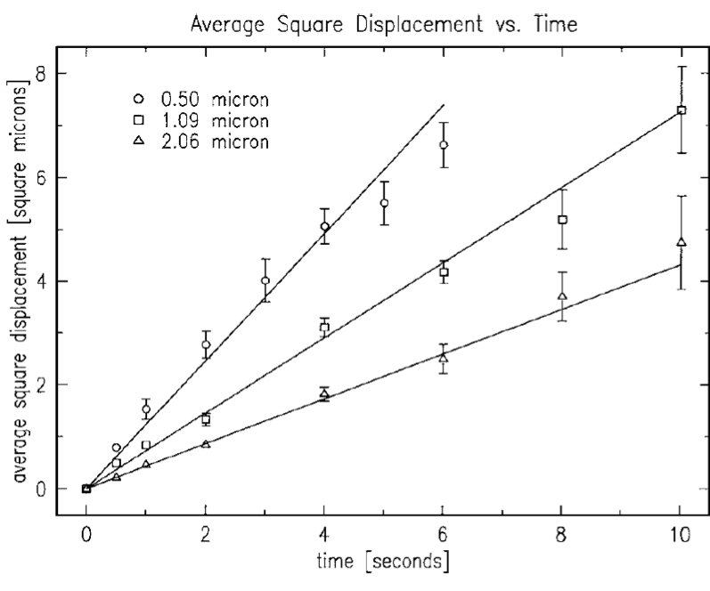
Performing this experiment in the 21st century was much simpler than it was for Perrin. Newburgh, Peidle, and Rueckner were able to purchase polystyrene microspheres of various sizes, eliminating the need to synthesize them. They also used a digital camera to record the particle positions over time instead of tracking the particles by hand. Using particles with radii of 0.50, 1.09, and 2.06 microns, they measured values of $latex 8.2 \times 10^{23}$, $latex 6.4 \times 10^{23}$, and $latex 5.7 \times 10^{23}$. Perhaps surprisingly, even with all of their modern advantages, the researchers’ results are not significantly closer to the actual value of $latex N_A = 6.02 \times 10^{23}$ than Perrin’s was a hundred years earlier.
Figure 2: Einstein’s relationship predicts that the mean square displacement should be linear in time. By observing this relationship for three different particle sizes, the researchers use the slope to obtain three measurements of Avogadro’s number. (Newburgh et al., 2006)
For those of us who work in the field of soft matter, the existence of Brownian motion and the linear mean square displacement of a particle undergoing such motion are well-known scientific facts. The authors of this paper remind us that, not so long ago, even the existence of molecules was not generally accepted. And, although we often take for granted that these results are correct, first-hand observations can be useful for developing a deeper understanding and appreciation: “…one never ceases to experience surprise at this result, which seems, as it were, to come out of nowhere: prepare a set of small spheres which are nevertheless huge compared with simple molecules, use a stopwatch and a microscope, and find Avogadro’s number.” [5]
[1] A. Einstein, “On a new determination of molecular dimensions,” doctoral dissertation, University of Zürich, 1905.
[2] J. Perrin, “Brownian movement and molecular reality,” translated by F. Soddy Taylor and Francis, London, 1910. The original paper, “Le Mouvement Brownien et la Réalité Moleculaire” appeared in the Ann. Chimi. Phys. 18 8me Serie, 5–114 1909.
[3] Avogadro’s number is the number of atoms or molecules in one mole of a substance.
[4] In 1908, three years after Einstein’s paper, Langevin also obtained the same result using a Newtonian approach. (P. Langevin, “Sur la Theorie du Mouvement Brownien,” C. R. Acad. Sci. Paris 146, 530–533 1908.)
[5] A. Pais, Subtle Is the Lord (Oxford U. P., New York, 1982), pp. 88–92.
In the beginning there was… what, exactly? Uncovering the origins of life is a notoriously difficult problem. When a researcher looks at a cell today, they see the highly-polished end product of millennia of evolution-driven engineering. While living cells are not made of any element that can’t be found somewhere else on earth, they don’t behave like any other matter that we know of. One major difference is that cells are constantly operating away from equilibrium. To understand equilibrium, consider a glass of ice water. When you put the glass in a warm room, the glass exchanges energy with the room until the ice melts and the entire glass of water warms to the temperature of the room around it. At this point, the water is said to have reached equilibrium with its environment. Despite mostly being made out of water, cells never equilibrate with their environment. Instead, they constantly consume energy to carry out the cyclic processes that keep them alive. As the saying goes, equilibrium is death[1]: the cessation of energy consumption can be thought of as a definition of death. The mystery of how non-equilibrium living matter spontaneously arose from all the equilibrated non-living stuff around ithas perplexed scientists and philosophers for the better part of human history[2].
An important job for any early cell is to spatially separate its inner workings from its environment. This allows the specific reactions needed for life, such as replication, to happen reliably. Today, cells have a complicated cell membrane to separate themselves from their environment and regulate what comes in and what goes out. One theory proposes that, rather than waiting for that machinery to create itself, droplets within a “primordial soup” of chemicals found on the early Earth served as the first vessels for the formation of the building blocks of life. This idea was proposed independently by the Soviet biochemist Alexander Oparin in 1924 and the British scientist J.B.S. Haldane in 1929[3]. Oparin argued that droplets were a simple way for early cells to separate themselves from the surrounding environment, preempting the need for the membrane to form first.
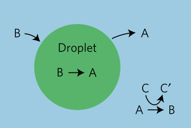
In today’s paper, David Zwicker, Rabea Seyboldt, and their colleagues construct a relatively simple theoretical model for how droplets can behave in remarkably life-like ways. The authors consider a four-component fluid with components A, B, C, and C’, as shown in Figure 1. Fluids A and B comprise most of the system, but phase separate from each other such that a droplet composed of mostly fluid B exists in a bath of mostly fluid A. This kind of system, like oil droplets in water, is called an emulsion. Usually, an emulsion droplet lives a very boring life. It either grows until all of the droplet material is used up, or evaporates altogether. However, by introducing chemical reactions between these fluids, the authors are able to give the emulsion droplets in their model unique and exciting properties.
Fig. 1: Model schematic. A droplet composed mostly of fluid B (green) within a bath of fluid A (blue). Inside the droplet, B degrades into A. Outside the droplet, fluids C and A react to form fluids B and C’. Adapted from Zwicker and colleagues.
The chemical reactions in the model are fairly simple (see figure 1). Fluid B spontaneously degrades into fluid A and diffuses out of the droplet. While fluid A cannot easily turn back into fluid B (since spontaneous degradation implies going from a high energy state to a low one), fluid C can react with A to create fluids B and C’, and this fluid B can diffuse back into the B droplet.
$latex B \to A \quad \text{and} \quad A+C \to B+C’$
If C and C’ are constantly resupplied and removed, respectively, they can be kept at fixed concentrations. Without C and C’, the entire droplet would disappear by degrading into fluid A, reaching equilibrium. Here, C and C’ act as fuel that constantly drives the system away from equilibrium, creating what the authors dub an “active” emulsion. Active matter systems like this one have had success in describing living things because they, like all living matter, fulfill the requirement of being out-of-equilibrium.
Because the equations that describe how fluids A and B flow over time are so complicated, the authors solve their model using a computer simulation. When they do, something remarkable happens. Emulsions with no chemical reactions with their surrounding fluids never stop growing as long as there is more of the same material nearby to gobble up. This process is called Ostwald ripening[4]. The authors find that an active emulsion system, due to the fact that material is constantly turning over, suppresses Ostwald ripening and allows the emulsion droplet to maintain a steady size.
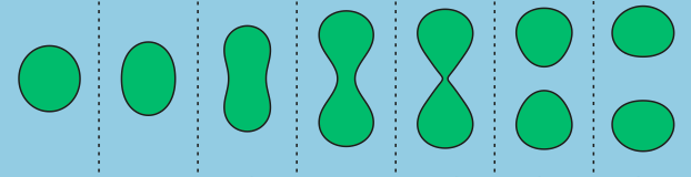
In addition to limited growth, the authors also find that the droplets undergo a shape instability that leads to spontaneous droplet division (see this movie). This occurs due to the constant fuel supply of C and C’. The chemical reaction A+C ? B+C’ creates a gradient in the concentration of fluids A and B outside the droplet. Just outside the droplet, there is a depletion of B and an abundance of A, while far away from the droplet, A and B reach an equilibrium concentration governed by the rate of their reactions with C and C’. The authors dub this excess concentration of B far away from the droplet the supersaturation. Where there exists a gradient in the concentration of a material, there exists a flow of that material, called a flux. This is the reason a puff of perfume in one corner of a room will eventually be evenly distributed around that room. The size of the droplet is dependent on the flux of fluid B into and out of the droplet.
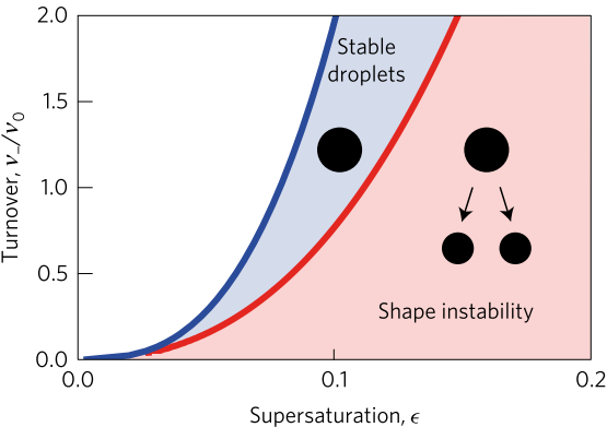
Two quantities determine the evolution of the droplet. The first is the supersaturation that reaches a steady value once all fluxes stop changing in time, and the second is the rate at which the turnover reaction B?A occurs. For a given supersaturation and turnover rate, the authors can calculate how large the droplet will grow, and they find three distinct regimes. In one regime, the droplet dissolves and disappears as the turnover rate outpaces the flow of fluid B back into the droplet. Another has the droplet grow to a limited size and remain stable, since the turnover and supersaturation balance each other out and give a steady quantity of fluid B. The third and most interesting regime occurs if the droplet grows beyond a certain radius due to the influx of fluid B outpacing its efflux. Here, a spherical shape is unstable and any small perturbation will result in the elongation and eventual division of the droplet (Figure 2).
Fig. 2: Stability diagram of droplets for normalized turnover rate $latex \nu_-/\nu_0$ vs supersaturation $latex \epsilon$. For a given value of $latex \epsilon$, the diagram shows regions where droplets dissolve and eventually disappear (white), grow to a steady size and remain stable (blue), and grow to a steady size and begin to divide (red). Adapted from Zwicker and colleagues.
And that’s it. If you have two materials that phase separate from each other, coupled to a constant fuel source to convert one into the other, controlled growth and division will naturally follow. While these droplets are more sophisticated than regular emulsion droplets, they are still a far cry from even the simplest microorganisms we see today. There is no genetic information being replicated and propagated, nor is there any internal structure to the droplets. Further, the droplets lack the membranes that modern cells use to distinguish themselves from their environments. An open question is whether a synthetic system exists that can test the model proposed by the authors. Nevertheless, these active emulsions provide a mechanism for how life’s complicated processes may have gotten started without modern cells’ complicated infrastructure.
Though many questions still remain, Zwicker and his colleagues have lent considerable credence to an important, simple, and feasible theory about the emergence of life: it all started with a single drop.
[1]: This isn’t exactly true. Some organisms undergo a process called anhydrobiosis, where they purposefully dehydrate and rehydrate themselves to stop and start their own metabolism. Also, some bacteria slow their metabolism to avoid accidentally ingesting antibiotics in a process called “bet-hedging”.
[2]: For example, ancient Greek natural philosophers such as Democritus and Aristotle believed in the theory of spontaneous generation, eventually disproven by Louis Pasteur in the 19th century.
[3]: Oparin, A. I. The Origin of Life. Moscow: Moscow Worker publisher, 1924 (in Russian), Haldane, J. B. S. The origin of life. Rationalist Annual 148, 3–10 (1929).
[4]: Ostwald ripening is a phenomenon observed in emulsions (such as oil droplets in water) and even crystals (such as ice) that describes how the inhomogeneities in the system change over time. In the case of emulsions, it describes how smaller droplets will dissolve in favor of growing larger droplets.