The trajectories of pointy intruders in sand

Original article: Collisional model of energy dissipation in three-dimensional granular impact

An alien spaceship commander was preparing to drop a cone-shaped spy shuttle into the sand of a Florida beach near Cape Canaveral. The shuttle needed to burrow deep enough that any passing humans wouldn’t see it while the aliens used it to spy on Earth’s space program. “From how high should I drop the shuttle so that it is hidden?” the commander asked their science advisor. The science advisor pulled out their alien high school mechanics book, hoping to calculate this based on the laws of motion and Earth’s gravitational force.

Not so fast, alien science advisor! While the mechanics of a falling shuttle are relatively simple, the forces the shuttle would experience while penetrating the sand are much more complicated. Sand and other granular materials are composed of millions of individual solid particles that, together, may be stiff like a solid or flow like a fluid. This interstellar scientist first needed to know how sand particles interact with one another and how the uneven distribution of forces between them before dropping the cone-shaped probe.

In “Collisional model of energy dissipation in three-dimensional granular impact”, C. S. Bester and R. P. Behringer asked a similar question. In their study, they looked at the forces that a conical object (such as the alien commander’s spy shuttle) experienced as it penetrated a granular material and investigated how these forces affect the depth a conical object will burrow. 

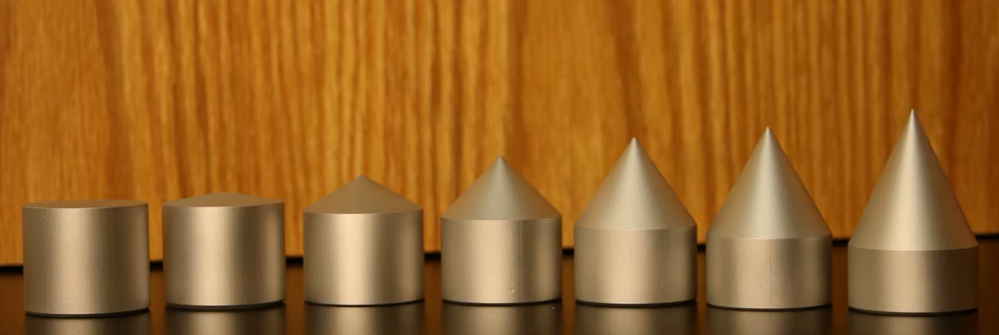
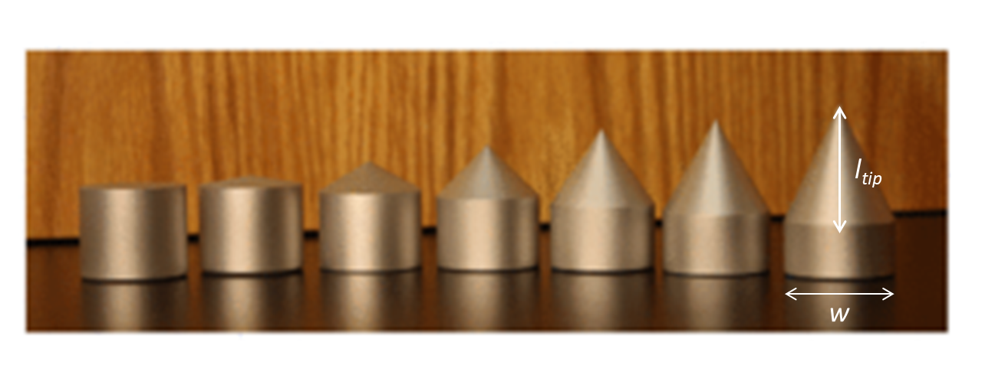
Bester and Behringer dropped conical intruders into a container filled with sand with a thin rod attached to the top of the intruder for tracking.  They filmed each falling intruder from the side with a high speed camera, from which they determined the depth z, velocity, and acceleration as the intruder penetrated the sand. For a video of the experiment, see here. They used the seven intruders shown in Figure 1 . The intruders all had the same mass m but different shapes. The sharpness of the intruder’s cone-shaped tip was characterized by a parameter s= \frac{2 L_{tip} }{w}, the ratio of its length to half its width. A higher value of s corresponded to a sharper cone. They were dropped from a range of heights between 6 cm and 2 m, which resulted in intruders reaching different speeds upon impact with the sand.

An image of seven intruders used in the experiment, ranging from a blunt intruder to an intruder with a conical top.
Figure 1: intruders of equal mass used in the experiment, from the bluntest (s = 0) to the sharpest (s = 2.1). Image adapted from original article.

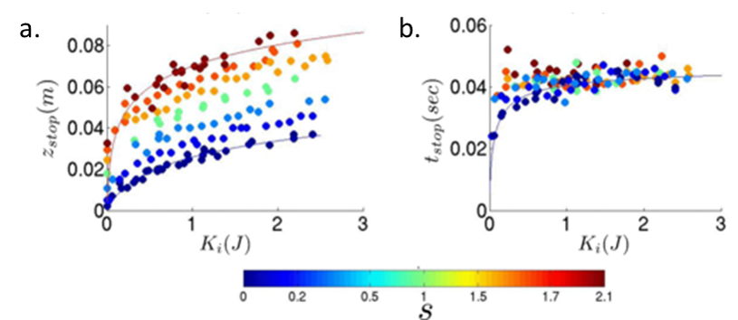
Bester and Behringer measured the stopping depth zstop and the time to stop tstop as a function of the initial kinetic energy each intruder had upon hitting the sand, K_i = \frac{1} {2}m z_i. They found that sharp intruders penetrated deeper into the sand than blunt intruders with the same kinetic energy Ki, as shown in Figure 2a. Figure 2b shows that, above an initial kinetic energy of 1 J, the time the intruders took to stop was the same regardless of shape or initial energy. 

Graphs of stopping depth as a function of kinetic energy and stopping time as a function of kinetic energy.
Figure 2: (a) Stopping depth as a function of kinetic energy. (b) Stopping time as a function of kinetic energy. Blue represents blunt intruders while red represents sharp intruders. Figure adapted from original article.

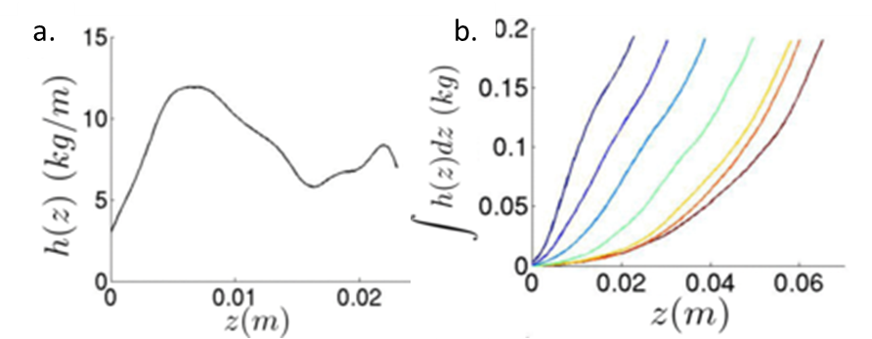
To understand what forces the intruder experiences as it comes to a stop, the authors focused on the inertial drag, or the drag caused by the pressure of the sand on the intruder.  Previous studies hypothesized that the inertial drag depended on the penetration depth and was proportional to the velocity squared of the intruder as it enters the granular material.  Bester and Behringer found that this was not the whole story. They calculated the inertial drag coefficient h(z) from the intruder trajectories, as shown in Figure 3a. Surprisingly, they found that the drag coefficient oscillated as the intruder penetrated the material. This suggested that the inertial drag was caused by collisions of the intruder with particles that are part of “force chains”. Force chains in a granular material are made up of connected particles that bear the majority of the forces in the material (see this earlier Softbites post for a detailed description). When the intruder hit a force chain, the drag increased due to the added resistance. The drag then decreased again when the chain was broken.

To investigate how the drag force was affected by the shape of the intruder, Bester and Behringer used the sum of the drag coefficient as the intruder penetrated the sand \int {h(z) dz} [1]. Blunt intruders had a drag that increased nearly linearly with depth, while the dependence of drag on depth was much more curved for sharp intruders, as seen in Figure 3b. The authors suggested that the nonlinear drag for sharper cones was caused by the changing surface area interacting with the grains. Upon impact, a sharp cone only interacted with the sand through the tip. As it sunk, the area that was in contact with the sand increased nonlinearly, which resulted in larger drag.  

Plots of the drag coefficient vs. height, showing a bumpy curve, and the drag dependence on the depth of different intruders, showing that the drag experienced by  sharper intruders has a nonlinear relationship with depth.
Figure 3: (a) Drag coefficient h as a function of height z for an intruder shows fluctuations. (b) Drag dependence on depth for different intruders. The drag of blunt intruders has a roughly linear relationship with depth (blue curves) while that of sharp intruders has a nonlinear relationship with depth (yellow and red curves). Figure adapted from original article.

Bester and Behringer’s investigation into how the shape of a conical intruder falling into sand affects the forces it experiences is a beautiful example of how complex the interactions of everyday materials can be. According to their work, the aliens in our introduction should drop a pointy probe from very high up to make sure it gets buried — and also put some sensors on their probe to measure how its descent is interrupted by the force chains in the sand.  The aliens may have imaginary science fiction technology that allows them to traverse light years, but even they may marvel at the countless collisions that affect the path of something they drop on the beach once they reach the Earth.


[1] The sum of the drag coefficient  (\int {h(z) dz}) was calculated from the measured kinetic energy, and then the derivative of it was taken to obtain the drag coefficient h. Taking the derivative amplified the noise in the measurement.  Bester and Behringer compared the sum \int {h(z) dz}. for different intruders to avoid this amplified noise.

Fold and Unfold

Animation of GFP unfolding

Original Paper: Mechanically switching single-molecule fluorescence of GFP by unfolding and refolding

For the most part of biology, it is form that follows function. Proteins are a perfect example of this — they are made of a sequence of amino acids (the protein building units), which are synthesized by the ribosome. Once synthesized, the long strings of amino acids fold up into a particular 3D shape or conformational state. Proteins take less than a thousandth of a second to attain their preferred conformational state (called “native state”) that — if nothing goes wrong — ends up being the same for a given sequence. This process is called protein folding. Explaining how a protein finds its folding preference out of all possible ways in such a short time is a longstanding problem in biology.

But, how do scientists know if – and when – a protein is in its folded state? The most straightforward way to do this is by observing its function — the way that a protein performs some biochemical task within the cell. If the protein is functionally active, then it has achieved its proper structure. However, most proteins are too small to observe directly without damaging the cell. To solve this problem researchers frequently use Green Fluorescent Protein (GFP), a protein that glows when it is hit by light of a specific wavelength. By attaching GFP to other proteins, researchers can see exactly where those proteins are at different timepoints. GFP’s stability, lack of interaction with other proteins, and non-toxicity make it an extremely popular candidate for visualizing protein localization. In other words, one “function” of GFP is to fluoresce. Today’s paper seeks to understand how structure correlates with function in GFP, one of biology’s most important tools.

To control the folding process, the authors used dual optical tweezers to mechanically stretch and relax the protein. Optical tweezers — as the name suggests — manipulate the position of particles (beads) using laser light. These beads are typically in the size range of micrometers. To apply forces on the GFP, the beads are attached to the protein via DNA “handles,” so that a DNA strand attached to the protein will stick to the DNA strand attached to the bead. These strands are then bound together ensuring that the force on the beads is transferred to the GFP. The construct looks as follows:

BeadDNAProteinDNABead

When the beads move apart, the protein is stretched to its maximal possible length (also called its contour length) and is unfolded, but when the beads get closer together, the protein folds back to its preferred structure. This process is illustrated in Figure 1.

Animation of GFP unfolding
Figure 1: The beads (circles) at each end are manipulated by laser beams and move back and forth. The DNA handles (purple) are attached to the GFP protein (green) that folds and unfolds turning to a functionally active and inactive state, respectively.

The authors observed that during unfolding, the GFP protein has undergone two intermediate states before unfolding completely. After unfolding, the beads were brought closer together and the protein folded itself back through the intermediate stages. The GFP molecule stopped emitting light when it was unfolded, which was expected. However, it started fluorescing only when it was completely in its folded state. This important finding showed that this protein is functionally inactive in any of the intermediate folding stages. The authors also observed that this process is reversible; they could unfold and refold the GFP molecule multiple times (see Figure 2).

Correlation between Fluorescence and Contour Length of the protein
Figure 2: Fluorescence signals of the GFP protein as it cycles through the unfolding and folding states. (A) The unfolded protein (light gray line) emits very little light (green signal) and its length fluctuates (purple line). Once the protein refolds (*) it emits more light and its length becomes shorter and consistent (dark gray line). † is the point where the force and state conformation are correlated(B) Cycled transition from dark (unfolded) to bright (folded). The purple circles represent the average contour length of each time. (Image adapted from Ganim’s and Rief’s paper).

These findings contribute towards understanding the functionality of proteins that could be used as in vivo optical sensors in force transduction. This work also opens up new avenues in studying biomolecules at the single-molecule level, such as DNA-protein complexes that can induce changes in conformation. Although the experiment only pulled the protein along one axis, this technique could be extended to pulling in several directions at once. If one could control the applied force in 3D, then it could be possible to gain more information on how exactly the protein folds and/or what happens during that process.

What is soft matter?

Keiser et al. & Lutetium Project

Look inside a glass of milk. Still, smooth, and white. Now put a drop of that milk under a microscope. See? It’s not so smooth anymore. Fat globules and proteins dance around in random paths surrounded by water. Their dance—a type of movement called Brownian motion—is caused by collisions with water molecules that move around due to the thermal energy. This mixture of dancing particles in water is called a colloid.

Colloids are one of the classic topics in soft matter, a field of physics that covers a broad range of systems including polymers, emulsions, droplets, biomaterials, liquid crystals, gels, foams, and granular materials. And while I can keep adding items to this list, I can’t give you a precise definition for soft matter. I’ve never seen a completely satisfying definition, and I’m not going to even attempt to provide that here. But I can give you a taste of some of the definitions, and I hope you’ll come away with the feeling that you sort of know what soft matter is.

The phrase “soft matter” brings to mind pillows and marshmallows. These things fall under physicist Tom Lubensky’s definition (given in a 1997 paper) of soft materials as “materials that will not hurt your hand if you hit them.” And while many materials in soft matter are too squishy to hurt you, some of them might—cross-linked polymers can be pretty hard. And what about colloids? Slapping milk won’t hurt, but it also seems strange to call milk soft.

To understand what the “soft” refers to in “soft matter”, we first have to know where the name came from. The French term “matière molle” was coined in Orsay around 1970 by physicist Madeleine Veyssié, who worked in the research group of one of the founding fathers of soft matter, Pierre-Gilles de Gennes. The phrase apparently started as a private joke within the de Gennes group (don’t ask me what it meant), and the English translation of “soft matter” was popularized by de Gennes in a lecture he gave after winning the Nobel prize in 1991. De Gennes wrote that soft matter systems have “large response functions”, meaning that they undergo a large (don’t ask me how large) change in response to some outside force. So it seems we’re meant to take “soft” to mean something closer to “sensitive”, not necessarily soft in a tactile sense.

Now we can think about why colloids are soft from a different perspective. Remember that milk droplet under the microscope? The fats and proteins move around in the droplet due to thermal energy in the water; they are “sensitive” to the forces caused by thermal energy.

But even this “large response functions” idea doesn’t describe everything in soft matter. Some topics often considered a part of the field are concerned with general mathematical concepts instead of particular materials or systems. Take, for example, particle packing—the way particles arrange themselves to fit into confined spaces. Studying how particles can be arranged to pack on a curved surface is a mathematical problem and isn’t directly related to large response functions. However, since classic soft matter systems such as colloids are made up of particles you might want to pack, it makes sense to include packing as part of the field.

For every definition you give for soft matter, you can find a system that doesn’t quite fit. In an APS news article from 2015, Jesse Silverberg described soft matter as “…an amalgamation of methods and concepts” from “physics, chemistry, engineering, biology, materials, and mathematics departments. The problems that soft matter…examines are the interdisciplinary offspring that emerge from these otherwise distinct fields.” So maybe it’s not that important to have a rigid definition for soft matter; maybe its indefinability should be part of its definition. Soft matter is a field where the lines between traditional scientific disciplines are becoming ever more blurred—or, rather, soft.


Image credits: Marangoni bursting from the Lutetium Project video and Keiser et al. PRL 2017. 2017 APS/DFD Milton van Dyke Award Winners.


Sticky light switches: Should I stay or should I go?

Original paper: Adhesion of Chlamydomonas microalgae to surfaces is switchable by light


One day it’s fine and next it’s…” red? Microscopic algae depend on photosynthesis, so they follow the light. Previous research has shown that their swimming is directed towards white light but not to red light. New work shows that light-activated stickiness allows microscopic algae to switch between different movement methods.

This indecision’s buggin’ me” – should I stick or should I swim? Different types of motility are needed to move through different environments. Microscopic algae live in a variety of different conditions, including soils, rocks, and sands, all surrounded by water. In general, we can split these conditions into two groups: those where the algae move within the water, or those where the algae move across a surface. Today’s paper studies how a unicellular algae changes from its free swimming state to a surface attached gliding state.

swimglide2008.png
Figure 1: Left: Chlamy’s normal swimming beat pattern, with different colors showing different time points. The cell body is shown in blue and the eyespot in red. Image adapted from [1]. Right: Gliding Chlamy moves due to proteins moving within the flagella. Image adapted from [2].
Kreis and co-workers investigate the unicellular green algae called Chlamydamonas reinhardtii, or Chlamy for short. It has two whip-like arms, called flagella, that it uses to move. In the swimming state, the flagella beat in a breaststroke to pull the cell forward, as shown in Figure 1A. In the gliding state, the flagella are stuck to a surface and the transport of proteins inside each flagellum pulls on the surface so the Chlammy moves across the surface, as shown in Figure 1B.

micropipetteFM2008
Figure 2: In micropipette force microscopy a small glass tube holds the cell. A surface (the substrate) can then be moved towards or away from the cell. The deflection of the micropipette as this occurs determines how sticky the cell is. All of this is done in water, where Chlamy lives normally. Image adapted from Kreis and coworkers’ paper.

To transition between these two movement methods, the Chlamy must attach and detach from the surface. The researchers measure the force Chlamy exerts on a surface when it attaches using micropipette force microscopy, shown in Figure 2. This method uses a micropipette, which is a small glass tube, to hold a single Chlamy cell in place with suction. The surface is moved towards or away from the cell, deflecting the micropipette from its original position based on the force the cells exert on the surface. The relationship between deflection distance and force is measured beforehand with calibration experiments. So, during the experiment, micropipette deflection yields how strongly cells are stuck. To understand how this force relates to the two movements methods, let’s look at the results.

frontandback2008
Figure 3: Adhesion force as a function of distance from the surface to the cell. The surface is initially 20 micrometers away from the cell and is moved closer, so the cell and surface touch. As the surface is moved away again we can see if the flagella-facing cell (a) or the back-facing cell (b) attach to the surface from the adhesion force that is built up. Figure adapted from Kreis and coworkers’ paper.

Figure 3 shows two force measurements, one where the flagella are facing the surface and another where the back of the cell is facing the surface. When the surface touches the flagella or back of the cell body, the micropipette is first deflected upwards, giving a positive force. As the surface is moved away, the micropipette moves back to its original zero-force position.

As the surface is moved further away, the flagella-facing cell and back-facing cell behave differently. The flagella-facing cell deflects the micropipette downwards, shown by the build-up of a largely negative force, whereas the back-facing cell does not deflect the micropipette and no force is exerted. This means that the flagella-facing cell sticks to the surface, whereas the back facing cell does not stick.

pullandgraph1009
Figure 4: Top row – left to right shows successive images of Chlamy pulling itself towards a surface – dashed red line shows the movement of the micropipette. The flagella are marked by solid red lines. Bottom row – micropipette deflection over time as the light is turned on and off as indicated by the arrows. Figure adapted from Kreis and coworkers’ paper.

The flagella not only stick but actively pull themselves towards the surface. At the top of Figure 4, we see the flagella touch the surface during their swimming beat cycle. First, just a small part of one flagellum is stuck to the surface. Then, the flagella actively pull themselves towards the surface until both are completely stretched out and ready for gliding. This process is reversible: as the light is turned on and off, so is the adhesion force. The Chlamy can pull themselves up again and again – transitioning between their stuck and free state.

difflight2008
Figure 5: Force-distance curves for the retraction of a surface under different wavelengths of light. The flagella only stick when shorter wavelengths of light are present. Figure adapted from Kreis and coworkers’ paper.

But what controls the transition? To answer this, the researchers repeated the experiment under different wavelengths of light. In Figure 5, we see that the stickiness peak is absent for red and green light but present for blue and purple light. Two potential light sensors could be responsible. One is on the cell’s eyespot and controls cell swimming to guide the cell towards the light. The other is on the flagella and controls the cell life cycle and several aspects of the cell’s mating process. But we don’t yet know which light sensor controls the stickiness, or which specific proteins make the flagella sticky.

So for the Chlamy, the decision to stay or go is made by checking if the lights are on! If they ‘go’ they can seek lighter environments, and if they ‘stay’ they can bask in the sunny spot. Watching Chlamy cells stick and un-stick as we flick a light switch is very cool, but why should we care about Chlamy? Chlamy is used in bioreactors to create biofuels and other bioproducts. Stuck Chlamy prevents light and nutrients from getting to all the cells in the reactor, so we need to understand how to control the sticking process. Plus – if we understand how a simple unicellular organism solves the problems of life, we can use this bio-inspiration for new technologies – in this case possibly new light-switchable adhesives.


[0] Should I Stay or Should I go?

[1] Antiphase Synchronization in a Flagellar-Dominance Mutant of Chlamydomonas

[2] Intraflagellar transport drives flagellar surface motility

From errant to coherent motion

Original paper

Emergence of macroscopic directed motion in populations of motile colloids. By Bricard A., Caussin J-B, Desreumaux N., Dauchot O. & Bartolo D.


Have you ever seen those wide shapes moving in the sky at dawn, made of thousands of starlings, or the swarms of fish swimming in the ocean (see Figure 1)? The ability to organize and move in groups without a leader is called collective motion and has been observed at various spatial scales in the living world, from birds to locusts, cells, and bacteria. Even humans can perform collective motion in some situations, as it has been modeled in crowd movements (for example Mosh pits). Physicists have gazed at this phenomenon over the last couple of decades trying to answer questions such as: How can different organisms exhibit the same behavior? What common features do all these organisms have that allow them to move in such a synchronized way?

The key to the emergence of collective motion is interactions, the ability of individuals to modify their behavior to coordinate their movements with those of their neighbors. The details of these interactions are difficult to model and control in many living or man-made systems, or may even still be unknown. Yet, in today’s paper, Antoine Bricard and colleagues showed how collective motion can arise solely from known physical interactions.

birds_fishes
Figure 1. Examples of collective motion in nature. (a) a flock of starlings (image adapted from howitworksdaily.com), (b) a swarm of fish (image adapted from scielo.br).

One of the first scientists who tackled these questions was Tamas Vicsek in the 90’s. He showed how collective motion can emerge from simple rules using a computer simulation. Although numerous theoretical and numerical studies followed, only few experiments were done. The biggest difficulty in studying collective motion experimentally is gaining control and reproducibility over a living system. Raising thousands of birds in a lab might not be the most convenient way of study, and even simpler biological systems, like bacteria, have problems of their own. Luckily, if you don’t want to deal with a biological system, you can build an artificial one. This is what Antoine Bricard and collaborators did, at Ecole Normale Supérieure de Lyon. To study collective motion, they built an artificial system made of millions of tiny, plastic beads (5 µm diameter) that were able to move freely, interact with their neighbors, and even self-organize as a group.

To put these inert beads in motion, researchers used a phenomenon called Quincke electro-rotation. The idea is to convert electrostatic energy into mechanical rotation. Here, the rotation is triggered by an electric field, E_0, applied to insulating beads, which are immersed in a conductive liquid. Under this field, small fluctuations in the charge distribution tilt the orientation of the bead. Then, the small rotational perturbation is amplified, resulting in a constant rotation and the bead rolling on the bottom of a pool. The researchers refer to these activated beads as “rollers”. All rollers move at the same speed, directly controlled by E_0, yet they don’t move in the same direction but rather randomly. As you can see in Figure 2, the beads move individually in different directions and there is no general directed motion. So how can this disordered system switch to an ordered motion?

Figure quincke
Figure 2. (a) The propulsion mechanism of a bead under an electric field, E_0, inducing an electric polarization, P. When P is tilted, the bead starts to rotate and moves forward at a constant speed, v. (b) A superposition of 10 images taken at successive timesteps showing the trajectories of 4 rollers activated by the Quincke electro-rotation. (Image adapted from the Antoine Bricard and coworkers’ paper.)

Using Quincke electro-rotation, the exact interactions between the rollers were described by the research team mathematically. Firstly, the beads interact through electrostatics, like two magnets, via an interaction that depends on how far they are from each other. Secondly, the beads interact through hydrodynamics, because when a bead moves in a liquid a flow is generated around it. This generates a pull similar to a swimmer who is feeling the flow produced by another swimmer nearby. What’s more, the theory shows that the combination of these two physical interactions tends to align a group of rollers. When two beads are close enough to each other, they slightly change their course to roll in the same orientation and they all eventually move in the same direction.

To study rollers for millions of particle lengths, the researchers chose to put them in a racetrack-shaped area (Figure 3 a). The rollers spontaneously organized, and a large band made of millions of rollers moved around the track. Of course, rollers had to be close enough in order for interactions to be effective. Figures 3 b-d show how the rollers changed behavior as they get more densely packed. In Figure 3 b, the rollers look like they are wandering in random directions because they are too far from each other to interact, while in Figure 3 d high-density rollers move in the same direction. And as more rollers are added in the same area, the interactions between rollers become more effective. This transition from a disordered state to an ordered state is called a phase transition. In most familiar cases, for example, water-to-ice, phase transitions are driven by temperature. Here density is the control parameter, meaning the research team measured what is the minimum density required for a collective motion to emerge. And being able to couple this observation with a theoretical description of the interactions, the key ingredient underpinning of the system, is what got them further than anyone else at the time.

Figure 3
Figure 3. (a) The racetrack band (watch the movie here) made of millions of self-organized rollers circulating around the area. (b-d) Screenshots of rollers at different densities; (b) at low density, (c) at the front of the band, and (d) at high density of rollers (watch the close view here). (Image adapted from the Antoine Bricard and coworkers’ paper.)

Collective motion seems natural in many living organisms but is still poorly understood by scientists. This paper highlights the importance of interactions between individuals in a group during the process of collective motion. Even though this study is specific and does not account for the mechanisms at work in most biological systems, it was a great achievement toward understanding this phenomenon. Comparing these results with the studies of biologists, ethologists, and mathematicians make me wonder: if a scientist working in his/her lab is like a random walker, then, what beautiful picture will emerge from the work of thousands of scientists interacting with each other to understand collective motion?

Putting the controversy over atomic-molecular theory to rest

Original paper: Einstein, Perrin, and the reality of atoms: 1905 revisited


There are many things that we “know” about the world around us. We know that the Earth revolves around the Sun, that gravity makes things fall downward, and that the apparently empty space around us is actually filled with the air that we breathe. We take for granted that these things are true. But how often do we consider whether we have seen evidence that supports these truths instead of trusting our sources of scientific knowledge?

Students in school are taught from an early age that matter is made of atoms and molecules. However, it wasn’t so long ago that this was a controversial belief. In the early 20th century, many scientists thought that atoms and molecules were just fictitious objects. It was only through the theoretical work of Einstein [1] and its experimental confirmation by Perrin [2] in the first decade of the 20th century that the question of the existence of atoms and molecules was put to rest. Today’s paper by Newburgh, Peidle, and Rueckner at Harvard University revisits these momentous developments with a holistic viewpoint that only hindsight can provide. In addition to re-examining Einstein’s theoretical analysis, the researchers also repeat Perrin’s experiments and demonstrate what an impressive feat his measurement was at that time.

In the mid-1800s, the botanist Robert Brown observed that small particles suspended in a liquid bounce around despite being inanimate objects. In an effort to explain this motion, Einstein started his 1905 paper on the motion of particles in a liquid with the assumption that liquids are, in fact, made of molecules. According to his theory, the molecules would move around at a speed determined by the temperature of the liquid: the warmer the liquid, the faster the molecules would move. And if a larger particle were suspended in the liquid, it would be bounced around by the molecules in the liquid.

Einstein knew that a particle moving through a liquid should feel the drag. Anyone who has been in a swimming pool has probably felt this; it is much harder to move through water than through air. The drag should increase with the viscosity, or thickness, of the fluid. Again, this makes sense: it is harder to move something through honey than through water. It is also harder to move a large object through a liquid than a small object, so the drag should increase with the size of the particle.

Assuming that Brownian motion was caused by collisions with molecules, and balancing it with the drag force, Einstein determined an expression for the mean square displacement of a particle suspended in a liquid. This relationship indicates how far a particle moves, on average, from its starting point in a given amount of time. He concluded that it should be given by

\langle \Delta x (\tau) ^2 \rangle = \frac{RT}{3 \pi \eta N_A r} \tau

where R is the gas constant, T is the temperature, \eta is the viscosity of the liquid, N_A is Avogadro’s number [3], r is the radius of the suspended particle, and \tau is the time between measurements [4]. With this result, Einstein did not claim to have proven that the molecular theory was correct. Instead, he concluded that if someone could experimentally confirm this relationship, it would be a strong argument in favor of the atomistic viewpoint.

A man using a camera lucida to draw a picture of a small statue.
Figure 1: A camera lucida is an optical device allows an observer to simultaneously see an image and drawing surface and is therefore used as a drawing aid. (Source: an illustration from the Scientific American Supplement, January 11, 1879)

This is where Perrin came in. Nearly five years after Einstein’s paper was published, he successfully measured Avogadro’s number using Einstein’s equation, confirming both the relationship and the molecular theory behind it. However, with the resources available at the time, this experiment was a challenge. Perrin had to first learn how to make micron-size spherical particles that were small enough that their Brownian motion could be observed, but still large enough to see in a microscope. In order to measure the particles’ motion, he used a camera lucida attached to a microscope to see the moving particles on a surface where he could trace their outlines and measure their displacements by hand. Perrin obtained a value of N_A = 7.15 \times 10^{23} by measuring the displacements of around 200 distinct particles in this way.

Performing this experiment in the 21st century was much simpler than it was for Perrin. Newburgh, Peidle, and Rueckner were able to purchase polystyrene microspheres of various sizes, eliminating the need to synthesize them. They also used a digital camera to record the particle positions over time instead of tracking the particles by hand. Using particles with radii of 0.50, 1.09, and 2.06 microns, they measured values of 8.2 \times 10^{23}, 6.4 \times 10^{23}, and 5.7 \times 10^{23}. Perhaps surprisingly, even with all of their modern advantages, the researchers’ results are not significantly closer to the actual value of N_A = 6.02 \times 10^{23} than Perrin’s was a hundred years earlier.

A plot of the average mean square displacement of three different sized particles over time.
Figure 2: Einstein’s relationship predicts that the mean square displacement should be linear in time. By observing this relationship for three different particle sizes, the researchers use the slope to obtain three measurements of Avogadro’s number. (Newburgh et al., 2006)

For those of us who work in the field of soft matter, the existence of Brownian motion and the linear mean square displacement of a particle undergoing such motion are well-known scientific facts. The authors of this paper remind us that, not so long ago, even the existence of molecules was not generally accepted. And, although we often take for granted that these results are correct, first-hand observations can be useful for developing a deeper understanding and appreciation: “…one never ceases to experience surprise at this result, which seems, as it were, to come out of nowhere: prepare a set of small spheres which are nevertheless huge compared with simple molecules, use a stopwatch and a microscope, and find Avogadro’s number.” [5]


[1] A. Einstein, “On a new determination of molecular dimensions,” doctoral dissertation, University of Zürich, 1905.

[2] J. Perrin, “Brownian movement and molecular reality,” translated by F. Soddy Taylor and Francis, London, 1910. The original paper, “Le Mouvement Brownien et la Réalité Moleculaire” appeared in the Ann. Chimi. Phys. 18 8me Serie, 5–114 1909.

[3] Avogadro’s number is the number of atoms or molecules in one mole of a substance.

[4] In 1908, three years after Einstein’s paper, Langevin also obtained the same result using a Newtonian approach. (P. Langevin, “Sur la Theorie du Mouvement Brownien,” C. R. Acad. Sci. Paris 146, 530–533 1908.)

[5] A. Pais, Subtle Is the Lord (Oxford U. P., New York, 1982), pp. 88–92.

Are squid the key to invisibility?

Original paper: Adaptive infrared-reflecting systems inspired by cephalopods


While many today would associate a “cloak of invisibility” with Harry Potter, the idea of a magical item that renders the wearer invisible is not a new one. In Ancient Greek, Hades was gifted a cap of invisibility in order to overthrow the Titans, whereas, in Japanese folklore, Momotar? loots a straw-cloak of invisibility from an ogre, a story which is strangely similar to the English fairytale Jack the Giant-Slayer. Looking to the future in Star Trek, Gene Roddenberry imagined a terrible foe known as the Klingons, a war-driven race that could appear at any moment from behind their cloaking devices – indeed, any modern military would bite your arm off to get hold of this kind of device. Clearly, invisibility is a concept that has captured minds across many cultures, genres, and eras, so it should be no wonder that scientists are working on making it a reality.

As is often the case in materials science, a good starting point for inspiration is to look to biology, after all, life has had billions of years of competition-driven evolution to craft its tools. To that end, Gorodetsky and his team at of the University of California, Irvine, have been attempting to replicate the master of disguise: the cephalopod. From this class of mollusk, squid and octopuses in particular excel at adaptively altering the color, texture, and patterning of their skin to camouflage against a wide variety of oceanic backdrops (see Figure 1). They accomplish this primarily by stretching and contracting pigment-containing skin cells. More importantly to this research, some species of squid have additional skin cells called ‘iridocytes’, which are structured reflective cells that resemble a microscopic comb or folded pleats. These folds reflect light at specific wavelengths that correspond to the fold size. By actively stretching and contracting these cells on-demand, the squid effectively becomes a self-modifying bioelectronic display.

SquidCamouflage (1)
Figure 1: Squid before (left) and after (right) deploying camouflage. Images reproduced from
a video by H. Steenfeldt under the YouTube Creative Commons Attribution license.

Following this technique of stretch-induced camouflage, the authors devise a technique for replicating some squid-like properties in an artificial material. The procedure consists of using electron-beam evaporation[1] to deposit an aluminum layer onto a stretched polymer film held under strain. When they release the strain, the metallically coated material shrinks and buckles to form microscopic wrinkles that are analogous to the structures in squid iridocyte cells. The polymer film of choice is an excellent proton conductor, so when mounted to electrodes, it can be stretched back to the flat state simply by applying a voltage.

When stretched, the aluminum coated film will reflect infrared light like a perfect mirror, whereas when wrinkled, the incoming light is reflected diffusively in multiple directions, like sunlight hitting the moon. To see this effect, the scientists shine infrared light – a heat source – at the material and position an infrared camera at a specific angle so that when flat, it reflects all the incoming radiation toward the camera and appears hot; when relaxed and wrinkled, much less of the light is scattered towards the camera, making the material appears to take on the thermal properties of the background and disappear from view.

Perhaps as a head-nod to their biological inspiration, the team then recreate this material in the likeness of a squid and watch as its infrared silhouette disappears from the camera’s view (Figure 2).

InfraInvisibleSquidShape_Fixed (1)
Figure 2: The flexible squid-shaped material, viewed under an infrared camera. When relaxed (left), very little infrared is reflected towards the camera, and it appears cold. When stretched (right), it reflects most incoming infrared light towards the camera and appears hot. Image edited from Fig. 5 in the manuscript.

The authors conclude that this ready-for-manufacturing material will have immediate applications in heat-regulating technology, and while it is currently limited to the infrared part of the spectrum, they also note that there is no reason why this technique couldn’t be adapted to the optical range.

Squid haven’t solved our desires for a cloak of invisibility just yet, but these mysterious creatures may hold more secrets than we realize. We would be wise to keep an eye on them … if we can.


[1]  Electron beam evaporation is the technique of bombarding a solid metal with energetic electrons, causing it to evaporate. This metal vapor then cools and condenses uniformly on all nearby surfaces, forming a uniform metallic coating.


Elastogranularity and how soil may shape the roots of plants

Original paper: Elastogranular Mechanics: Buckling, Jamming, and Structure Formation


How an elastic beam deforms under load has been a question for as long as there have been engineers to ask it. In some cases, the force on a beam is approximated as a single point. For example, if a diving board is large enough, a diver at the end can be treated as a point mass on the beam. Another common approximation is to consider the force to be a continuous pressure along its length. Treating wind that bends a tree branch as a continuous pressure along the branch’s length is much simpler than adding up the force from every molecule of air on the branch. However, consider the case of a root growing into a granular material like soil. As the root burrows through the soil it will bend due to varying point-like forces along its length. The result is a branching and twisting root system that tries to grow along the path of least resistance. An example of the diversity in plant root morphologies is shown in Figure 1 and gives a sense of how complicated and interesting the physics behind this growth can be.  

Figure 1. An example of the complex and diverse morphology of several types of plants which all live in the same ecosystem [1]

With this in mind, David J. Schunter Jr. et al. from the Holmes group at Boston University have developed a beautiful experiment to study what they call “elastogranular” phenomena. In their experiment, an elastic beam is inserted into a box which is filled at a particular density with uniform beads. An image of a typical experiment is shown in Figure 2. Once the beam reaches the end of the box it will not be able to penetrate any further, and trying to push more of the beam into the box will cause a compression along the beam’s length. This resembles a classic experiment where a beam is compressed in the same manner, but in the absence of beads. Compressing the beam against the end of the box becomes increasingly difficult until eventually the beam “pops” into one large buckle. In this simpler case, the beam was free to buckle with no restrictions. Introducing beads to the system reinforces the beam non-uniformly and constrains the shapes it can take on when it buckles. This complicates the buckling event and leads to interesting new behaviors.

Screenshot 2018-05-11 at 6.13.31 PM.png
Figure 2. An elastic beam is inserted into a box of length L_{0} and width 2W_{0} filled with beads at an initial packing fraction of \phi_{0} = 0.89. After a length of beam is inserted equal to L_{0}, inserting additional length \Delta results in buckling. In this experiment the beam takes on two buckles with wavelength \lambda, and amplitudes of A_{0} and A_{1} respectively.

In the experiment performed by the Holmes group, a beam is compressed against the end of the box until the beam buckles. If the packing fraction \phi_{0} (the fraction of space within the box that is covered in beads) is low, it buckles much like one would expect in the absence of beads—one large buckle, as in Figure 3i. If \phi_{0} is higher at the beginning of the experiment, like in Figures 3ii and 3iii, the buckling behavior becomes more complicated. The beam will form one large buckle as before, and as the buckle grows it will take up more area on one side of the box. This forces the beads to reorganize themselves, and the beads on the compressed side of the box become very tightly packed. At this point, they are in a hexagonal arrangement, and they are said to have crystallized [2]. As the beads in one side crystalize, that side becomes stiffer and suppresses further growth of the amplitude of the first buckle, A_{0}. In order to accommodate the extra length being inserted, \Delta, an additional buckle forms. The difference in buckling behavior for three values of \phi_{0} are shown in Figure 3. [3]

Figure 3. Shape profiles of the inserted rod for various packing fractions (\phi_{0}) for the same normalized inserted length \Delta/L_{0}. i) At low \phi_{0} the beam forms one large buckle. ii) As \phi_{0} increases, the amplitude of the single buckle is suppressed, leading to a second buckle forming on the other side. iii) At even higher \phi_{0}, the buckles rotate and grow toward each other.

Figures 3 shows that not only are the number and amplitude of buckles significantly affected by the beads that surround the beam, but the orientations of the buckles are changed as well. When the experiment begins at a high \phi_{0}, the beam finds both sides of the box to be stiff and hard to penetrate. The initial buckle does not grow very much before the second buckle forms, and at high enough \phi_{0} both buckles occur nearly simultaneously, forming a twin buckle. Figure 4 shows two systems with different \phi_{0} forming twin buckles. In the top sequence where \phi_{0} is lower, the buckles maintain a constant distance between each other as they grow since there are plenty of uncrystallized areas (light blue circles) ahead of the buckles into which they can grow. The lower sequence shows that, at higher \phi_{0}, the majority of uncrystallized beads are found in the wake of a buckle so the buckles instead grow into these regions, as demonstrated by the red lines.

Figure 5. Twin buckles increase in amplitude as \Delta increases (left to right) growing into less-dense, uncrystallized regions (light blue circles). For lower \phi_{0} (top sequence), uncrystallized beads in front of the buckles can be pushed aside, crystallizing beads away from the buckles (dark blue and yellow circles). At higher \phi_{0} (lower sequence), the uncrystallized sections occur behind the buckles, causing the two buckles to grow closer together which is shown by the red lines.

This system bears a striking resemblance to that of plant roots growing into the soil and could be useful in understanding how environmental pressures cause plant root systems to evolve. For example, cacti need to absorb as much water as they can from their environment. One way of accomplishing this is to increase the surface area of the root system by growing wide and close to the surface, rather than deep, in order to collect water from a larger area. By developing thin roots that buckle before they can deeply penetrate the soil, many cacti are able to produce the shallow, wide-reaching roots system they need to find water.

David J. Schunter Jr. and coworkers have shown that combining two well-understood problems—buckling of a beam and reorganization of beads—can lead to unique and interesting bending dynamics. By confining a beam to a box of beads, the buckling of the beam becomes strongly influenced by the packing fraction and reorientation of the beads. This particular system shows a strong resemblance to plant root growth, but also be informative for synthetic applications involving the insertion of flexible filaments into deformable materials.


[1] Michigan Natural Shore Partnership, http://www.mishorelinepartnership.org/plants-for-inland-lakes.html

[2] When spheres crystallize in two dimensions, the hexagonal lattice is the closest possible packing with an area fraction of \phi = 0.9069. Interestingly, Figure 3iii shows a packing fraction of 0.91, which is higher than this maximum value. This is because the beads are able to pop out of the plane at very high compressions, which can lead to a calculated packing fraction larger than that of the hexagonal lattice. For more information on hexagonal packing, see Wikipedia.

[3] For more information about the specifics of how the deformation of the beam is quantified, a summary of the analysis is available here.