Biological Materials at SICB 2019

It’s unusual to run a symposium as a PhD student, but anyone can do it! I was lucky to find a great mentor to guide me through the process. Together we organized 11 speakers, 2 workshops, and 11 poster presentations for a full day discussion on what soft matter, materials, and evolutionary biology have in common. From fire ants to spider silk, tooth enamel to lizard scales, and chemistry to computer science, there are lots of opportunities for soft-matter researchers to study biological questions.

The annual meeting of the Society for Integrative and Comparative Biology (SICB) is one of the core conferences for organismal biology. Originally called the “American Society of Zoologists,” the society changed its name to SICB in 1996 to emphasize the “integration” of different biological specializations. This commitment to interdisciplinary research made SICB the perfect home for my interest in biologically produced materials.

I’m interested in how biomaterials are created and diversify, a topic that draws on soft matter physics, mechanics, and evolutionary biology. There are a lot of exciting questions in this area, but because they are so interdisciplinary, there are not that many people who work on them. Interdisciplinary research often falls outside traditional departments and grant funding options, making these projects hard to design and run. They also require careful communication skills (if you talk to an engineer and an evolutionary biologist about the “evolution of a biomaterial” you might get two very different answers– the engineer might think of “material evolution” as a change during the material’s use (how does it respond to heat or light?), while the biologist might think about changes as the material developed with different organisms over millions of years). Nevertheless, I think interdisciplinary research questions are some of the most exciting and important, and luckily I’m not alone.

Together with my co-organizer, Dr. Mason Dean from the Biomaterials Department of the Max Planck Institute for Colloids and Interfaces, we organized the SICB symposium “Adaptation and Evolution of Biological Materials” (#AEBM #SICB2019) to highlight what is already being done in this field, and to encourage more biologists to start working with materials and soft matter.

Here are some highlights from our speakers:

Entanglement

Beyond “active matter” systems like fish schools or bird flocks, there are also collections of individual organisms that entangle together and behave like squishy, living materials. Prof. David Hu and Prof. Saad Bhamla presented on two different entangled soft matter systems: fire ant swarms and worm blobs. Both can act sometimes like a liquid and sometimes like a solid, depending on how the individuals link together. These systems can be described similarly to collections of molecules, complete with phase separation behavior!

Tunability

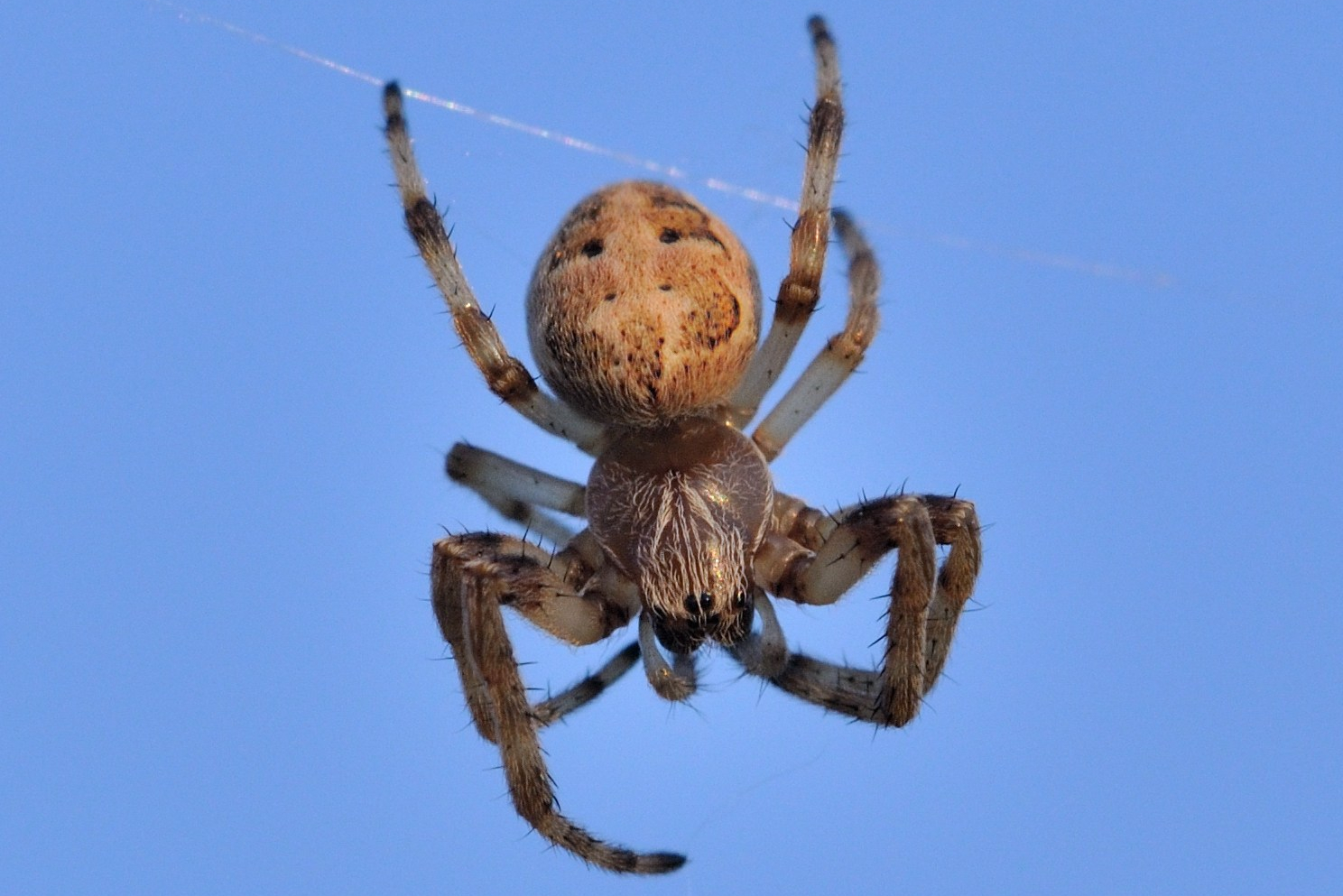
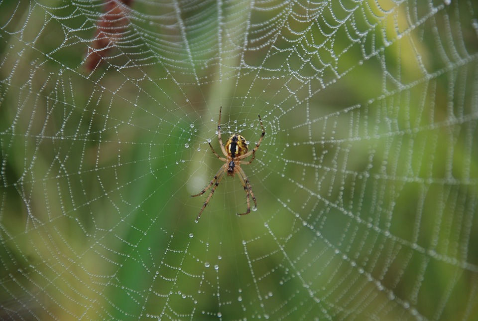
Unlike a lot of human-engineered systems, almost all biological materials have multiple functions. Dr. Beth Mortimer studies vibrational communication in spiders, worms, and elephants. Here she presented recent work suggesting the material vibration sensors built into spider legs might be tuned specifically for silk material properties — highlighting how silk has evolved to be both a structural and sensory material.

Assembly

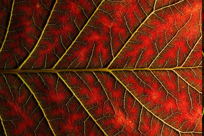
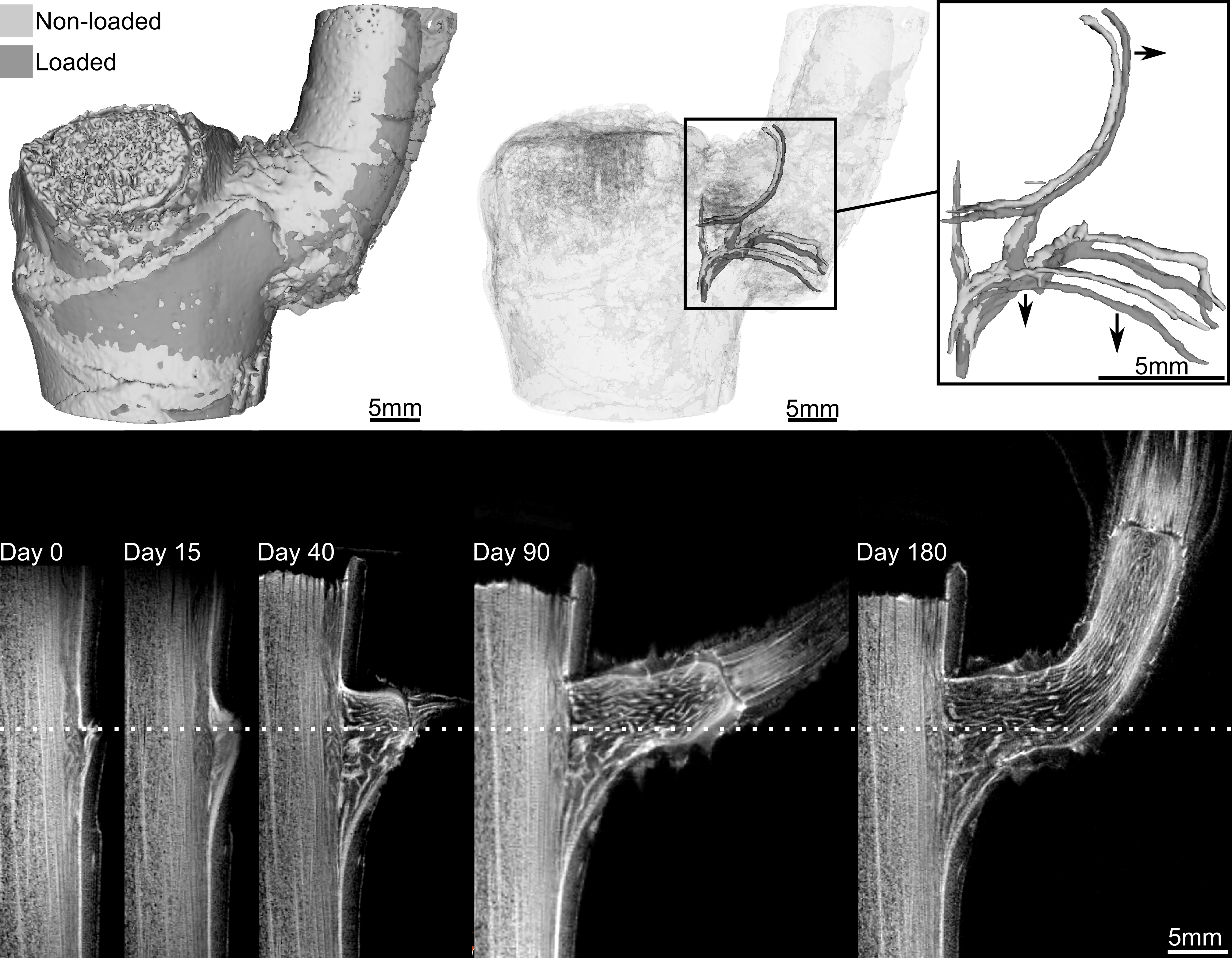
Biological materials are famous for being made of simple, individual components that can assemble into complex structures on their own (i.e. “self assembly” without a human engineer). We had a lot of talks referencing this topic. Dr. Linnea Hesse studies the joints of branching plants to try and learn why they are so sturdy. She found that the vascular bundles that transport water (the equivalent of human capillaries for blood flow) adapt to external forces as the branch grows. This way the bottom of the branch is arranged differently than the top to optimize load bearing.

plant-branch-loading
The organization of vascular bundles in the dragon tree changes during growth, making the joints between branches and the trunk stronger. (Image courtesy of Dr. Linnea Hesse)

On a smaller scale, Prof. Matt Harrington presented on a new model of fiber formation from the velvet worm. Velvet worms shoot slime at their prey, which quickly hardens into fibers with strength comparable to nylon. If that wasn’t cool enough, these fibers can be dissolved in water and then later resolidify! Making them an intriguing model for new biodegradable plastics. Unlike spider silk, which is made of tiny highly ordered fibers, the “silk” of the velvet work seems to be made of relatively disordered charge-stabilized droplets.

Last but not least, Dr. Ainsley Seago has surveyed the colorful nanostructured scales of hundreds of species in two lineages of beetles. Her results suggest that even though these surfaces exhibit many different optical properties, they’re all likely assembled as liquids in a process remarkably similar to the assembly of cell membranes (called lyotropic assembly).
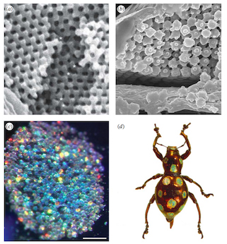
beetle-structural-color
The shiny, bright colors on beetles come from nanostructured scales. (Image courtesy of Dr. Ainsley Seago)

Image Analysis

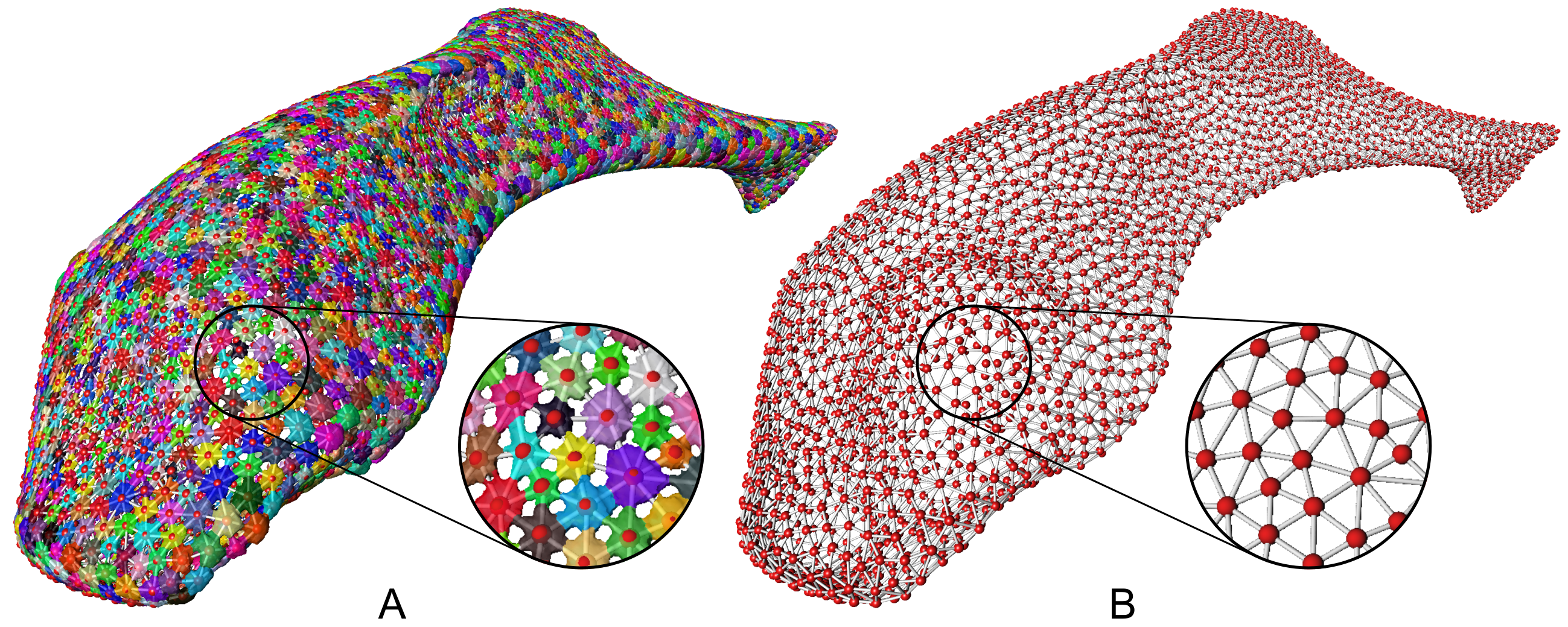
Dr. Daniel Baum is an expert on computational solutions for automated image analysis. He presented on common approaches for automatically selecting different parts of an image. This is really useful for studying material and biological systems with lots of similar repeating structures, and modeling how these systems respond to external forces. He presented examples of this work applied to the study of sharks and rays, whose soft cartilaginous skeletons are wrapped in a network of tiny, repeating, mineralized plates (called tesserae).

modeling-tesserae
Computational methods, such as the watershed algorithm, can automatically segment different parts of an image and be used to construct 3D models of bones, cartilage, and other material. (Image courtesy of Dr. Daniel Baum)

Hierarchy

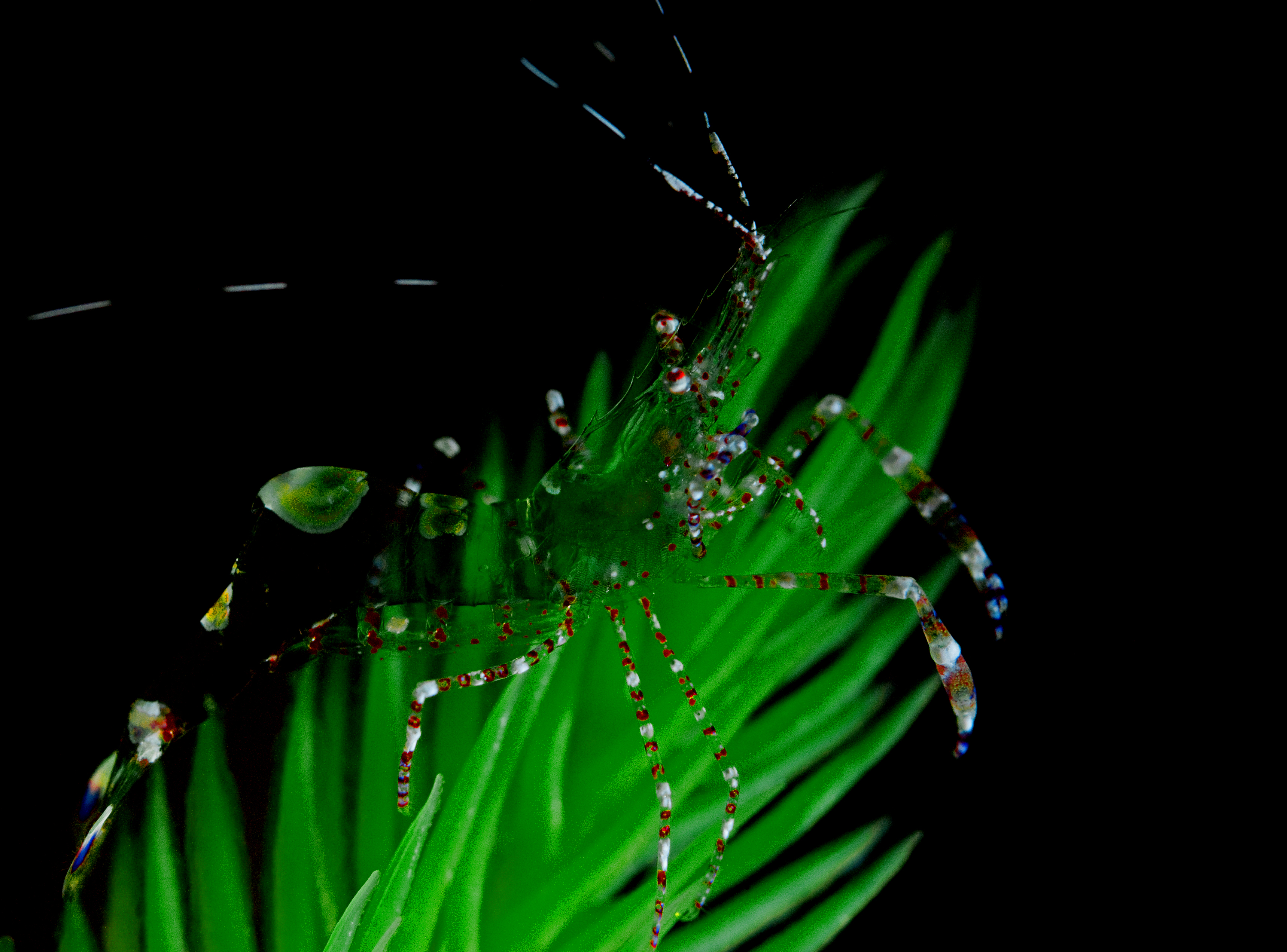
The layered organization of materials at different scales (forming a hierarchy of structure) is important for many biological materials’ properties. Dr. Laura Bagge studies invisibility in deep sea ocean life, and she presented how the size of the tiny microfibrils that make up larger muscle fibers can change how opaque an organism is — larger microfibrils have fewer interfaces for light to interact with, allowing the whole body of some shrimp species to be transparent.

These kinds of hierarchies are more commonly associated with strength, as in the example that Dr. Adam van Casteren presented. He studies how enamel, the outer layer of the tooth, resists wear, showing work suggesting that different levels of the material structure (nanostructure vs. microstructure) might respond differently to evolutionary pressure. That means that these hierarchies might have evolved to protect against damage from different types of diets, i.e. abrasion from sand particles in plant-based diets versus fracture from breaking apart bones and shellfish.

transparent-shrimp
Transparent shrimp achieve invisibility by having larger muscle microfibrils. (Image courtesy of Dr. Laura Bagge)

Microfluidics

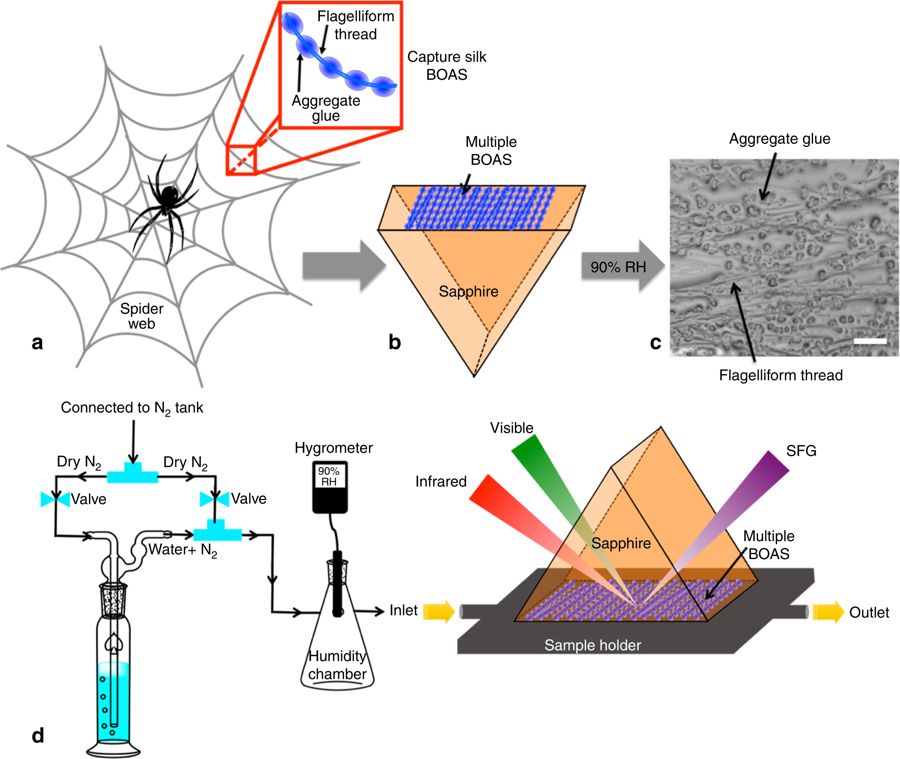
Fluid transport (both liquids and gases) is crucial for organism survival, so it’s no surprise that many biomaterials have been optimized for this function. Dr. Anna-Christin Joel presented work on how lizard scales and certain spider silks use capillary forces to manipulate fluids. The same capillary control has been harnessed to transport water droplets collected along the body to the mouth for drinking and to make capture silk stick more tightly to prey (by pulling waxes up from the surface of insects).

In a different application of fluid handling, Prof. Cassie Stoddard talked about the large eggs of emus. All eggs have pores that provide airflow to the growing chick, but the pores in emu eggs are forked not straight. This might help solve the challenge of getting enough breathable air into large eggs without weakening the shell enough that it could be crushed by the adult (interestingly this feature is also seen in dinosaur eggs!).

Spider silk: Sticky when wet

Original paper: Hygroscopic Compounds in Spider Aggregate Glue Remove Interfacial Water to Maintain Adhesion in Humid Conditions 


If you were Spider-Man, how would you catch your criminals? You could tangle them up in different types of threads, but to really keep them from escaping you would probably want your web to be sticky (not to mention the utility of sticky silk for swinging between buildings). Like Spider-Man, the furrow spider spins a web with sticky capture silk to trap its prey. This silk gets its stickiness from a layer of glue that coats the thread. What makes this capture silk really interesting is that, unlike commercial glues, these spider glues don’t fail when wet.

The tendency for water to interfere with glues should come as no surprise. For example, sticky bandages become unstuck when they’re wet, whether it’s because of swimming, taking a shower, or going for a run on a humid day. This interference occurs on the microscopic scale, where water prevents the components of a glue from forming adhesive chemical bonds. Even just high humidity provides enough water vapor in the air for it to condense on nearby surfaces and interfere with adhesion. One would naturally expect this very general and simple mechanism to cause problems for spiders that lay traps near water, as our furrow spider does. As you may have guessed, our furrow spider is a bit more clever than that: their glues are highly effective regardless of the water content of the air, and this humidity-resilience has caught the attention of Saranshu Singla and colleagues at the University of Akron, Ohio.

spider-516653_960_720
Figure 1. A spider unperturbed by the water droplets formed on its sticky web.

The furrow spider glue being studied by Singla and co-workers is essentially a cocktail of 3 main components: specialized “glycoproteins” that act as the primary adhesive molecule, a group of smaller low molecular mass compounds (LMMCs), and water. The LMMCs group covers a wide range of chemicals (both organic and inorganic), but the main distinguishing feature of this group is that they are hygroscopic, which means they are water absorbing. The exact recipe of this glue is specific to each spider species, and previous research has shown that individual species’ glues stick best in the climate that spiders evolved in—rather than humidity causing them problems, tropical spider webs are in fact most effective in humid conditions.

To understand how spiders achieve this, the researchers used a combination of spectroscopy [1] techniques to observe the arrangement of molecules during adhesion. They took a densely packed layer of web threads collected from the furrow spider and stuck them to one side of a sapphire prism, an ideal surface for its smoothness and transparency to the light rays used for spectroscopy (See Figure 1 for experimental schematic). They then measured the chemical bonds at the point of contact between the glue droplets and the sticking surface over a range of humidity conditions. These measurements allowed them to figure out what happens when these sticky glues get coated in water.

41467_2018_4263_Fig1_HTML
Figure 2. Experimental setup schematic from the manuscript. The white scale bar in c is 0.1 mm. Here “flagelliform” refers to the silk material prior to the glue layer being added, and “BOAS” refers to the classic beads-on-a-string structure that droplets form on threads. SFG stands for “sum frequency generation” spectroscopy, the noninvasive technique used in this research for analyzing the molecular arrangement at the sticking interface between the glue droplets and the sapphire surface.

Singla and her colleagues find that there is very little liquid water at the sticking interface, despite water being one of the three main glue elements. They concluded that the hygroscopic LMMCs are drawing water away from the droplet surface and storing it near the center. The LMMCs make it possible for the sticky glycoproteins to fulfill their role: in high humidity the glue droplet first absorbs nearby water, and then draws that water away from the droplet surface, preventing it from interfering with the sticky molecules’ adhesive chemical bonds. The researchers also conclude that the glue’s efficiency at drawing water to the center of the droplet is controlled by the local humidity and the ratio of the three components. Tweaking this ratio would then make the glue better adapted to different humidities. This suggests that the addition of hygroscopic compounds provides a simple method to tune adhesives to suit specific environments.

This continues to be an exciting time for materials science as scientists unlock the secrets of nature, but perhaps more importantly, Peter Parker can now rest easy with the knowledge that Humidity-Man will be a highly ineffective foe.


1. Broadly, spectroscopy is a study of the interaction between matter and light. There are many different types of spectroscopy, as there are many different ways that light and matter interact, but typically, a beam of light covering a range of the electromagnetic spectrum (hence the “spectro” prefix) is shone onto a substance, and then regathered by a light detector. The brightness of the detected light at each wavelength can then be used to carefully analyze the properties of the substance. Here, the researchers combined infrared spectroscopy and SFG, a non-invasive technique that is specifically tailored to probe molecular arrangements at interfaces, and so is perfectly suited for probing interfacial adhesion.

Scaling up biology

Original paper

A General Model for the Origin of Allometric Scaling Laws in Biology. By Geoffrey B. West, James H. Brown, and Brian J. Enquist. Science 1997


Physics is a discipline that attempts to develop a unifying, mathematical framework for understanding diverse phenomena. It connects things as different as planets orbiting the sun and a ball thrown through the air by showing that both these motions come from a single equation [1]. Living things do not seem to obey such simplicity, but hidden beneath all the diversity and complexity of life are remarkably universal patterns called scaling laws. In a landmark 1997 paper by Geoffrey West, James Brown, and Brian Enquist, a simple explanation is given for how all organisms, from fleas to whales to trees, can be thought of as non-linearly scaled versions of each other.

A scaling law tells you how a property of an object, say the rate at which energy is consumed by an organism (its metabolic rate), changes with the object’s size. Just by looking at the data, many quantities scale as a power law of the mass, 

$latex A \propto M^{\alpha}$    (Eq. 1)

where ? is some number that, from the data, always seems to be a multiple of 1/4 [2]. West, Brown, and Enquist build a theory showing how biology could have come up with this 1/4 power law, but in this article, I’m just going to focus on one specific example. I’m going to walk through the author’s arguments for how the metabolic rate, the rate at which an organism consumes energy, scales with an exponent of 3/4. They show that it all comes up from some basic assumptions about the networks that distribute nutrients to your body — your circulatory system [3].

These networks are assumed to have two characteristics [4]. First, they are space-filling fractals. Fractals are shapes made of smaller, repeating versions of themselves no matter how far you zoom into it. However, our fractal blood vessels can’t get arbitrarily small, they have a “terminal unit”— the capillary. The second assumption about these networks is that all terminal units are the same size, regardless of organism size. With these two assumptions, the authors are able to derive the 3/4 power law for metabolic rate.

Branching veins representing as a regular, branching network
Figure 1: Cartoon of a mammalian circulatory system on the left, which can be represented as a branching network model on the right. Adapted from Figure 1 of the original paper.

First, let’s build up a picture of what these networks look like. Figure 1 shows how the circulatory system can be thought of as a network structured into N levels, where each level k has $latex N_k$ tubes. At each level, a tube breaks into a number ($latex m_k$) of smaller tubes. Each one of these tubes is idealized as a perfect cylinder with length $latex l_k$ and radius $latex r_k$, as shown in Figure 2.

Tube parameters
Figure 2: Illustration of the different parameters that each tube on the kth level of the network has. Adapted from Figure 1 of the original paper

How does blood move through this network? Well, the blood flow rate at each level of the network must be equal to the blood flow rate at every other level. Otherwise, you would have the equivalent of traffic jams in your arteries. You don’t want those. If the blood flow speed through one tube in the kth level is $latex u_k$, the blood flow rate through the entire kth level is

$latex \dot{Q}_k = N_k \pi r_k^2  u_k = N_{cap} \pi r_{cap}^2 u_{cap} = \dot{Q}_{cap}$    (Eq. 2)

Your metabolic rate, B, depends on the flow rate through your capillaries, $latex \dot{Q}_{cap}$, so the authors assume that the two are proportional to each other: $latex B \propto \dot{Q}_{cap}$. Because all terminal units are the same size, the only variable left in Eq. 2 to relate to an animal’s mass is $latex N_{cap}$. Assuming that B scales like $latex B \propto M^{\alpha}$, and the authors predict

$latex N_{cap} \propto M^{\alpha}$    (Eq. 3)

branchingRatios-01
Figure 3: Schematic of a branching point along the network, illustrating the definitions of the ratios $latex \beta_k$ and $latex \gamma_k$. In this case, $latex m_k = 2$.

To figure out the value of the exponent $latex \alpha$, the key is to get $latex N_{cap}$, which depends on the size of the organism, in terms of the capillary dimensions $latex r_c$ and $latex l_c$, which do not. To do this, the authors use relations derived using the self-similar geometry of the fractal network. When a tube breaks into smaller tubes, it does so with a ratio between the successive radii, $latex \beta_k = r_{k+1} / r_k$, and another ratio between the successive lengths, $latex \gamma_k = l_{k+1}/l_k$. This is illustrated in Figure 3. Because the network is fractal, the number of tubes each branch breaks into,  $latex m_k$, the ratio of radii, $latex \beta_k$, and the ratio of lengths, $latex \gamma_k$, are all assumed to be constant for every k,

$latex \beta_k = \beta, \; \gamma_k = \gamma, \; m_k = m \;\; \forall k$

Since, at every level, each branch breaks into m smaller branches, the total number of capillaries (i.e. the number of branches at level N) is $latex m^N$. Plugging this into Eq. 3,

$latex \alpha = \frac{N \ln(m)}{\ln(M/M_0)}$    (Eq. 4)

Where  $latex M_0^{\alpha}$ is the proportionality constant between $latex N_{cap}$ and $latex M^{\alpha}$. Remember, we’re trying to show that $latex \alpha = 3/4$.

Now that $latex N_{cap}$ has been rewritten in terms of network properties, the authors next turn their attention to  another quantity that scales with the organism size — its mass, M. To do this, the authors use the empirical fact that the total volume of blood, $latex V_b$, is proportional to the total mass of the organism, $latex V_b \propto M$. The total volume of blood is given by:

$latex V_b = \sum_{k=0}^N V_k N_k = \sum_{k=0}^N \pi r_k^2 l_k m^k \propto \left( \gamma \beta^2 \right)^{-N} \propto M$    (Eq. 5)

In the above equation, the first proportionality sign (summing the series) requires a calculation that’s given here. The main idea of this calculation is that, because the ratios $latex r_{k+1} / r_k$ and $latex l_{k+1}/l_k$ are each constant, the sum in Eq. 5 can be turned into a geometric series which can be summed analytically. Plugging the final proportionality from Eq. 5 into Eq. 4,

$latex \alpha = – \frac{\ln(m)}{\ln(\gamma \beta^2)}$    (Eq. 6)

To make further progress, we have to know something about $latex \gamma$ and $latex \beta$. Every tube of the network gives nutrients to a group of cells. As every good physicist does, the authors will assume that this group of cells has the volume of a sphere with a diameter equal to the length of the tube. The volumes serviced by each successive level are approximately equal to each other,  $latex 4/3 \pi (l_{k+1} / 2)^3 N_{k+1} \approx 4/3 \pi (l_k / 2)^3 N_k$. From this, they get an expression for $latex \gamma$:

$latex \gamma_k^3 \equiv \left(\frac{l_{k+1}}{l_k}\right)^3 \approx \frac{N_k}{N_{k+1}} = \frac{1}{m}$    (Eq. 7)

which means

$latex \gamma \approx m^{-1/3}$

Now the authors move on to $latex \beta$. Earlier, I argued that the flow rate has to be the same from one level of the network to the next to avoid “traffic jams” of blood. Since the tubes are assumed to be perfect cylinders, this boils down to the idea that the cross-sectional area of a parent tube being equal to the total cross-sectional area of its daughter tubes, $latex \pi r_k^2 = \pi r_{k+1}^2 m$. From this, the authors find an expression for $latex \beta$:

$latex \beta_k^2 \equiv \left( \frac{r_{k+1}}{r_k} \right)^2 = \frac{1}{m}$     (Eq. 8)

Similar to the expression for $latex \gamma$, this means

$latex \beta \approx m^{-1/2}$

Plugging in the expressions for $latex \gamma$ and $latex \beta$ in terms of m, we finally arrive at our desired result:

$latex \alpha =  – \frac{\ln(m)}{\ln(\gamma \beta^2)} = – \frac{\ln(m)}{\ln(m^{-1/3}(m^{-1/2})^2)} = 3/4$    (Eq. 9)

What West and his colleagues have done is use the fact that all organisms have to deliver nutrients to their individual parts to derive a general, universal scaling law. The authors go on to show that when you add a pump to the system, such as our heart, the analysis may get more complicated, but the ultimate result remains unchanged. All living things, regardless of size, seem to have arrived at the same solution for nutrient supply, building systems that are space-filling, fractal, and have the same size “terminal units”. Turns out we’re not so different after all.


[1] $latex F = Gm_1 m_2 / r^2$. ^

[2] For example:

  • $latex \alpha = 3/4$ for cross section area of aortas of mammals, tree trunk sizes
  • $latex \alpha = -1/4$ for cellular metabolic rate, heartbeat rate, population growth
  • $latex \alpha = 1/4$ for time of blood circulation, life span, embryonic growth rate ^

[3] All the arguments hold for other distribution systems, such as our pulmonary system, plant vascular systems, and insect respiratory systems. ^

[4] There’s an additional assumption that the network is designed to minimize energy, but that won’t come into play in the part of the author’s arguments that I will be presenting here. ^