The dance of swarming flies

Original article: Emergent dynamics of laboratory insect swarms

Imagine yourself as a small fly called a midge (shown in Figure 1a). You used to live in a lake as a small larva with no concerns in life except swimming, eating, and growing. One day, you hid underwater and formed a cocoon around your body as it developed wings, legs, and antennae. A few days later, you swam to the surface and burst out of your cocoon as an adult fly — a male. As a new adult male, you find the clock ticking – you have only a few days to find a mate before you die.

Attracting a female is difficult for a tiny midge – how is she going to see you flying around? Fortunately, you can team up with hundreds of other male midges. Together, you fly above the lake in a stationary swarm that looks like a large cloud. Females can find this swarm and fly into it for their choice of mate. 

In today’s study, Douglas Kelley and Nicholas Ouellette investigate how the motion of midges in a swarm helps the swarm stick together.

Figure 1. (a) A midge is a tiny fly that forms mating swarms above lakes (image from Wikipedia). (b) Midges tracked in a swarm in the laboratory, with different midges in different colors (Figure adapted from original article)

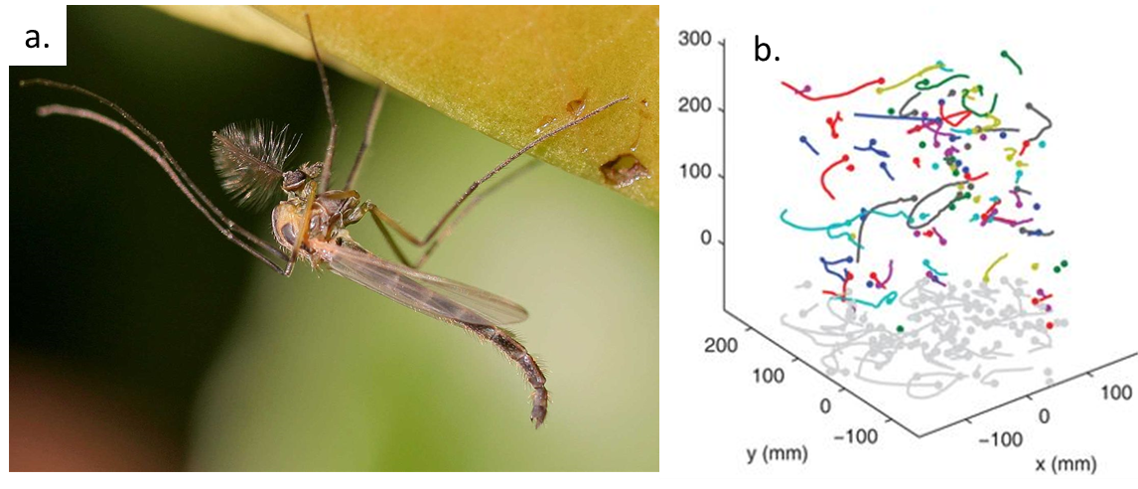
The researchers set up midge swarms in the laboratory and film them with three infrared cameras. They track all of the individual midges in the swarm and calculate their trajectories. Tracking dozens of small midges is not easy! First, they use the 2D images from the three cameras to locate the flies in 3D for each frame. Then, they use a technique originally developed for studying turbulent fluid flows to generate the trajectories over time. This technique uses the history of each midge to estimate where it is likely to be next and looks for midges in that area at the next time step. The resulting trajectories are shown in Figure 1b.  The positions, velocities, and accelerations of the midges give clues about how the swarm moves.

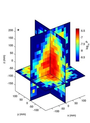
First, Kelley and Ouellette discuss the position of the midges. They plot the logarithm of the probability (log_{10} P) of finding a midge in a point in the swarm in three dimensions in Figure 2. Bright red represents a high probability of finding a midge, and blue represents a very low probability. Midge swarms are nearly symmetric, but larger swarms (of 100 individuals or more) are slightly taller than they are wide. This is unlike bird flocks, which are nearly two-dimensional.

Figure 2. Probability of finding a midge at x, y, and z coordinates in the swarm. Bright red colors indicate high likelihood of finding a midge, and blue represents a very low chance of finding a midge in that position. (Figure adapted from original article)

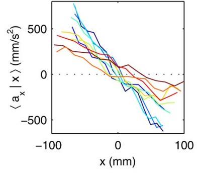
The researchers then investigate the velocities of the midges. Since the swarm is stationary, the average velocity of all the midges in the swarm is nearly zero. It turns out that the standard deviation, or the variation, of the velocities of the individual midges is more useful for understanding the motion inside the swarm. Midges fly twice as fast horizontally as vertically, just like birds in a flock. However, unlike flocks of birds, the midge swarms  are not polarized — a midge does not tend to fly in the same direction as its neighbors. Finally, Kelley and Ouellette investigate the acceleration of the midges in the swarm. The midges are equally likely to turn in any direction, unlike birds or fish. Relative to their body size, larger animals have more inertia than smaller ones, and must exert a lot more effort to turn, accelerate, and decelerate. Thus, they tend to keep moving in the direction they are currently moving. Midges, on the other hand, can turn and easily move in any direction. Kelley and Ouellette find the average acceleration of the midges in the swarm in the x-direction as a function of the midge’s x-position, \langle a_x|x \rangle, in Figure 3.  The midges tend to accelerate towards the center of the swarm, keeping the entire swarm together despite the midges’ constant motion. [1]

Figure 3. Acceleration of the midges in the x-direction as a function of the x-position for several midge swarms.  Each line represents a different swarm. When a midge is at the right edge of the swarm, it accelerates to the left (and vice versa).  (Figure adapted from original article)

In this study, Kelley and Ouellette quantify a new type of swarming behavior. Unlike most other animal aggregations like bird flocks and fish schools, midge swarms stay in one place, helping female midges find the love of their very short lives.


[1]  Surprisingly, when Kelley and Ouellette investigated the mean square displacement of the midges, they found that the midges act as if they are trapped in a box with walls.

A Storm of Oscillators

Original paper: Oscillators that sync and swarm


Japanese tree frogs follow a mating ritual that is so strange and beautiful that studying them may give rise to a new kind of science. During the rainy season, the male frogs gather near paddies and ponds and call to attract females. Researchers have found that isolated single male frogs call periodically [1], however, groups of males that are located near each other try to call out of sync. This temporal difference in calls allows the female frogs to correctly locate the male frogs. This is a natural system where spatial location of the frogs dictates the synchronization of their calls. This leads to an interesting question: What happens if you allow the synchronization of their calls to dictate their locations instead?

Scientists study synchronization to understand how an oscillating system evolves over time. However, systems ‘in sync’ do not usually move through space in a way that is related to their oscillations – consider the light flashes from a gathering of fireflies or the beating of a cardiac pacemaker. Swarming, on the other hand, is a form of self-organization where the participating individuals move through space, guided by some simple rules. In today’s paper by O’Keeffe, Hong, and Strogatz, the authors try to get a theoretical understanding of systems that show both synchronization and swarming. Previously, there had been studies of “mobile oscillators” where it was assumed that the location of an oscillator in space affected its phase. Here, the authors come up with a new theory that the phase affects where the oscillator is located in space. They name such particles swarmalators and propose a simple model to study their collective states analytically.

Imagine a set of particles on a plane, where each one is labeled by a number 1,2,3, etc. The ith particle (where i is any of the labels 1,2,3, etc.) has an internal state represented by a variable theta, \mathbf{\theta}_i, and a position represented by the vector \mathbf{x}_i. The internal state \mathbf{\theta}_i is equivalent to a phase angle, so it can only take on values between 0 and 2?, while \mathbf{x}_i can be any position on the plane. The key to swarmalators is that their position affects how their internal state changes and their internal state affects how their position changes. A relatively simple way to model this would be by the following set of equations:

\dot{\mathbf{x}}_i =  \frac{1}{N} \sum_{j \neq i}^{N} \frac{x_j-x_i}{|x_j-x_i|}(1+J cos(\theta_j-\theta_i)) - \frac{x_j-x_i}{|x_j-x_i|^2}

\dot{\mathbf{\theta_i}} = \frac{K}{N}\sum_{j \neq i}^{N}\frac{sin(\theta_j-\theta_i)}{|x_j-x_i|}

The most interesting parameters in these equations are J and K. Let’s step through the equations to see what their effects are. The first equation says how the position of the ith swarmalator changes in time, given by the time derivative of \dot{\mathbf{x}}_i. It is affected by all the other particles. The first term in the sum is an attraction between particles and points in the direction from particle i to particle j. The parameter J controls how oscillations lead to reorganization in space. For positive J, the closer two swarmalators internal states are, the more they attract since cos(x) is maximized around x = 0. When J is negative, swarmalators are attracted to swarmaltors with as different from an internal state as possible. When J = 0, swaramalators’ spatial movements are immune to other’s internal state. The second term is simply a repulsion between particles, preventing them from occupying the same place.

Similarly, the second equation says how the internal state (the phase angle) changes in time. Like the position, it has a constant angular velocity, \mathbf{\omega}_i, and is also affected by all the other particles. The parameter K represents how well the internal state of oscillations are synchronized for swarmalators. For a positive K, the swaramalators want to be synchronized with each other, while for negative K they want to oscillate out of phase. This effect is distance dependent, so swarmalators are more affected by nearby swarmalators than ones that are further away.

The authors use a computer to solve this pair of governing equations to see how such a system will evolve over time. They report that there can be five different states based on the two parameters J and K (Figure 1).

41467_2017_1190_Fig1_HTML
Figure 1: Diagram showing the various combinations of J and K which give rise to the various states of the model.

Static synchrony: For all positive K and all J, the model predicts that swarmalators will arrange themselves in a circularly symmetric manner. Each of the swarmalators will be fully synchronized in phase (Figure 2). All static states reach an equilibrium after some time.

41467_2017_1190_MOESM4_ESM
Figure 2: This animation shows the time evolution of swarmalators when they are in a state of static synchrony. All swarmalators occupy a disk and they all have the same phase.

Static asynchrony: For negative J and negative K, i.e. for cases when swarmalators want to oscillate out of phase but are attracted to opposite phases spatially, they are distributed uniformly and every phase occurs everywhere. (Figure 3).

41467_2017_1190_MOESM5_ESM
Figure 3: The animation shows how swarmalators evolve and rearrange themselves in the state of static asynchrony. The swarmaltors all occupy a disk, with phases different from their neighbors, leading to all phases existing everywhere.

Static phase wave: For the special case K=0 and J>0,.when the swarmalators’ phases are frozen in time but they like to settle near other swarmalators with the same phase, an interesting phenomenon occurs. Since positive J means “like attracts like” the swarmalators arrange themselves in regions of similar phases. This leads to an annular structure where the spatial angle of each swarmalator is perfectly correlated with its phase of oscillation (Figure 4).

41467_2017_1190_MOESM6_ESM.gif
Figure 4: The state of static phase wave where the spatial angle of the swarmalators is directly correlated to their phase of oscillation.

Splintered phase wave: In the K<0 half-plane, and when the magnitude of K is not too large, the swarmalators tend to oscillate out of phase weakly while trying to get closer to similar phases and a non-stationary state occurs. Here the particles keep rearranging themselves into disconnected clusters of distinct phases. Unlike the earlier static states, within each cluster, the swarmalators execute small amplitude oscillations in both position and phase about their mean values.

41467_2017_1190_MOESM7_ESM.gif
Figure 5: The splintered phase wave state.

Active phase wave: On decreasing K further — that is, when swarmalators strongly desynchronize but try to move towards swarmalators in sync — the oscillations in phase and position increase until the swarmalators start to execute regular cycles. Although this is a new phase, the authors point out that the motion of swarmalators is reminiscent of the double milling of biological swarms where the population splits into groups that are rotating in opposite directions.


41467_2017_1190_MOESM8_ESM.gif
Figure 6: Swarmalators showing an active phase wave.

In this paper, O’Keeffe and his colleagues have demonstrated how a system of particles that have the freedom to move in space and match the oscillation phase of their neighboring particles can lead to a rich variety of patterns that change in space and time. Perhaps most interestingly,  the authors claim that there is no known natural system where splintered phase waves and active phase waves occur. Thus, this paper provides an interesting lead for experimentalists searching for new patterns in nature.


[1] Mathematical modeling of frogs