simulation – Softbites

2018-12-052020-03-04

The Ketchup Conundrum and Molecular Dynamics: Unraveling the Mystery of Shear Thinning

Original paper: Structural predictor for nonlinear sheared dynamics in simple glass-forming liquids

We’ve all been there. We try pouring ketchup onto our fries from the bottle, but it doesn’t come out. So we tap the back of the bottle a few times, and suddenly, the ketchup rushes out and your entire meal is covered with it. Why does the ketchup exhibit such behavior?

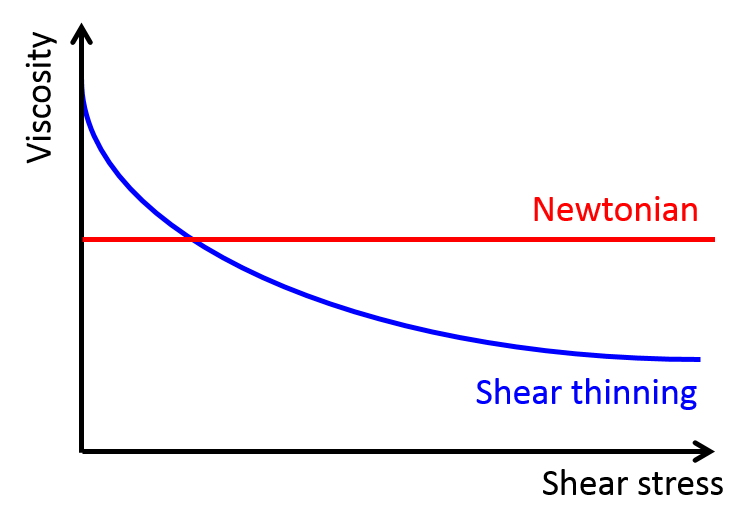
This behavior is called shear thinning, and only some special fluids exhibit it. For fluids, such as water and alcohol (these are called “classical” or “Newtonian” fluids) viscosity only depends on temperature. Therefore, if the temperature doesn’t change, the viscosity remains constant (see the red curve in Figure 1). However, in non-Newtonian fluids, viscosity depends on another variable called the shear stress. Shear stress is the stress felt by materials when they undergo deformation caused by slip or slide. In shear-thinning fluids, which are a type of non-Newtonian fluids, the viscosity decreases when the shear stress increases (see the blue curve in Figure 1). Ketchup, with other suspension fluids such as blood and nail polish, falls into this category of shear-thinning fluids. So, by tapping the ketchup bottle, we apply shear stress to the ketchup inside, causing the viscosity to drop and making the ketchup flow out of the bottle. But, even though this phenomenon has been on scientists’ radar for a long time, the microscopic mechanism for shear thinning is still unknown for certain fluids.

**Figure 1.** Shear stress vs. viscosity of Newtonian and shear-thinning fluids.

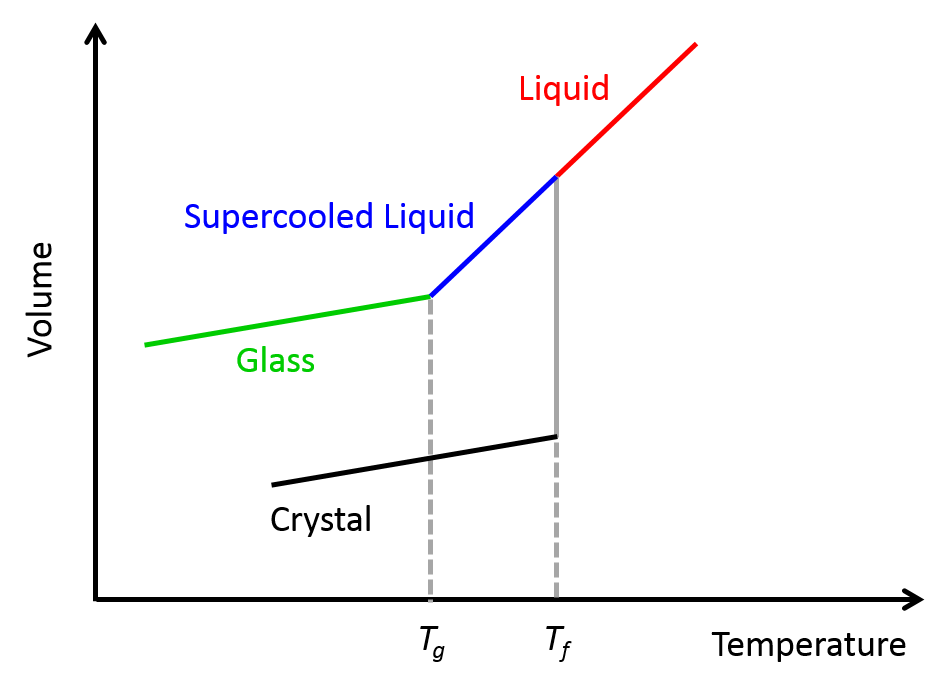
Another type of fluid that exhibits shear-thinning behavior is the “supercooled” liquids. As shown in Figure 2, when a liquid – any liquid – is rapidly cooled below its freezing point, instead of crystallizing and solidifying (like what we typically see when water freezes in an ice-cube tray), it forms a supercooled liquid. When the temperature of this highly viscous liquids drops even further below its glass-forming temperature, it turns into a disordered glass-like phase [1]. That is why supercooled liquids are also called glass-forming liquids.

**Figure 2.** The relationship between the volume of liquid and supercooled liquid. *T_f* and *T_g* indicate freezing point and glass-forming temperature, respectively.

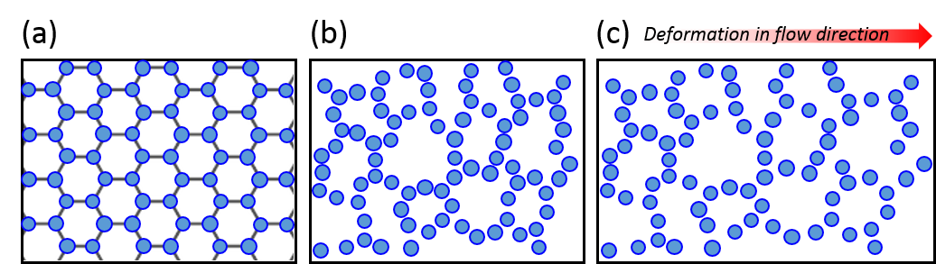
To understand the flow behavior of supercooled liquids, Trond Ingebrigtsen and Hajime Tanaka of the Institute of Industrial Science at the University of Tokyo ran molecular dynamics simulations. Molecular dynamics simulation is a computational method for studying the interactions of atoms or molecules. From the simulations, Ingebrigtsen and Tanaka were able to confirm what other scientists had previously suspected: shear thinning is linked to the increase in structural disorder of the liquid molecules (as illustrated in Figure 3(a) and 3(b)). To be more specific, it is linked to the structural disorder of molecules in the flow direction.

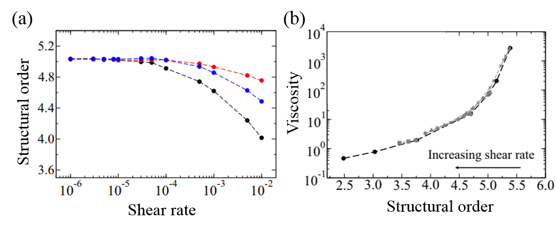
As a model for supercooled liquids, the authors chose to simulate a colloidal system, where molecules interact in a similar way to realistic fluids. After verifying that the simulates system acts like a supercooled liquid (for example, its viscosity decreases with increasing shear rate), they investigated the origin of shear thinning using this model. The molecular simulation revealed that as the shear rate increases, the molecular structure becomes more disordered. This is illustrated in Figure 3(a) and 3(b). More notably, the structural disorder was more prominent in the direction of the fluid flow compared to the structural disorder measured in any other directions relative to the flow. This can be seen from the black line of Figure 4(a), where the steep decrease of structural order could be observed with increasing shear rate.

Indeed, the structural disorder turned out to be the culprit behind the shear-thinning behavior in supercooled liquids. As shown in Figure 4(b), when the molecular structure becomes more disordered, the viscosity of the liquid decreases, a behavior expected in shear-thinning fluids. To understand this result, let’s picture molecules in the fluid. The shear applied in the direction of the flow would open up more space for molecules to rearrange themselves as the fluid expands, like it is shown in Figure 3(c). This leads to the decreased viscosity and the easier fluid flow.

**Figure 3.** (a) Structurally ordered molecular system. (b) A molecular system with increased disorder. (c) System after shear deformation in the flow direction.

**Figure 4.** (a) Shear rate versus structural order of the supercooled liquid model used in the molecular simulation. The black line represents the flow direction (blue and red each represents other two directions relative to the flow.) (b) Structural order versus viscosity. (Note the log scale on the y-axis.) All figures are adapted from the original paper.

This study sheds light on the previously unknown mechanism of shear thinning in supercooled liquids. Ingebrigtsen and Tanaka, however, insert that the microscopic mechanism for their observation should be further studied to fully understand the shear-thinning behavior. So, next time a disaster happens on your fries, chill out and think that you are just carrying out a super cool non-newtonian experiment!

(This post was updated on March 4th, 2020 to answer a comment that was made on the French translation of this post.)

[1] Technically, glass isn’t a phase, though I used that word for simplicity. Glass is an amorphous solid that has a disordered molecular structure (unlike ice, which has a well-defined crystalline structure). See Figure 3(b) for a visualization of a disordered molecular structure.

2018-06-132018-06-11

Imagine you are a Sea Slug Larva…

Original paper: Individual-based model of larval transport to coral reefs in turbulent, wave-driven flow: behavioral responses to dissolved settlement inducer

Lost, alone, and buffeted by ocean currents: this is the beginning of life for many oceanic larvae. These tiny organisms, often only 100 micrometers in diameter, must seek a suitable new habitat by searching over length scales thousands of times their own. But searching for something you can’t see while being dragged this way and that by ocean currents can’t be easy. How do these microscopic creatures make sense of the turbulent world around them and find their home?

larvaandslug — Figure 1: The larval form (left) is about 100 micrometers in diameter and swims using the beating hairs on the stumps on at the top of the cell, whereas and the adult sea slug form (right) can grow up to 5 cm in length and stays on the coral. Left figure is taken from Koehl et. al. The right figure is taken from http://www.seaslugforum.net/find/pheslugu.

To answer this question, today’s paper studies a species of sea slug, Phestilla sibogae. These sea slugs have two forms, the baby larval form (Fig. 1 left), which travels through the ocean, and the adult sea slug form (Fig. 1 right), which lives and feeds on their coral prey. After they are born, the young larvae first swim toward light, instinctively leaving their parents’ reef. When they are old enough to settle down and become adults, they must search for a new reef to call home. The metamorphosis from larva to slug is only triggered when the larvae have settled on their coral prey.

The coral prey release a chemical that the sea slug larvae can smell. The chemical acts as an on-off switch for the larva. When there is no chemical, the larva swims in a straight path in a random direction at 170 micrometers per second. Upon encountering a strong enough chemical smell, the larva stops swimming and sinks at 130 micrometers per second. We know how the larva move but how does this movement affect how many and how quickly the larvae make it to the reef? To understand the larvae transport, we need to understand the larval environment.

larvaeinsea — Figure 2: Larva cell (inset) in turbulent waters above the reef. The streaky pattern is from measurements made by the researchers in a wavy flow tank above a reef skeleton. Within the reef skeleton, a fluorescent dye is released. When the fluorescent dye is excited by a laser sheet it emits light. More light means more dye, where the dye represents the coral chemical [1]. The figure is taken from Koehl et. al.

Not only do the larvae have to swim while being buffeted by the wavy turbulent flow, but the waves also affect how the chemical released from the reef spreads. If the coral were in still water, then the amount of chemical would increase smoothly as you travel from the surface waters to the reef due to diffusion. However, the corals live in shallow water, where waves passing over the rough reef surface lead to turbulent waters above the reef. This complicated flow pattern means the chemical smell no longer smoothly increases as you travel towards to reef. Instead, the turbulence creates streaks of very high amounts of chemical and very low amounts of the chemical, as shown in Figure 2.

To investigate the transport of larvae to the reef, Koehl and coauthors build on previous work to create a computer simulation with both the larva swimming behavior and the larva environment based on experimental measurements. To model the background flow environment, they include the net flow, waves, and turbulence. The flow parameters are fit to experimental measurements made in wavy shallow waters in Hawaii [1]. In a similar way, the researchers use experimental measurements to model the swimming behavior of the larvae.

In their simulation, the researchers are able to alter both the environment and the larva swimming behavior and ask what, if any, advantage the on-off swimming behavior brings. The advantage is measured using the steady state larva transport rate, defined as the percentage of the larvae that make it to the reef each minute. With the steady-state approximation, the percentage of larvae that make it to the reef each minute is constant over time.

bothconcpatterns — Figure 3: Turbulent concentration pattern in A shows streaks of high and low concentration while the time-averaged concentration pattern in B smoothly increases towards the bottom of the reef. Figure adapted from Koehl et. al.

First, the researchers investigate whether or not the streakiness of the concentration pattern is an important factor in determining how many larvae reach the coral. When trying to understand how larvae reach the coral, previous researchers made the simplifying assumption that the concentration pattern of the chemical the larvae follow is smooth and uniform over time. As we saw in the streaky pattern in Figure 2, this is not a realistic assumption. But just how wrong is this it? To answer this question, the researchers compare the chemical distribution measured at a single moment in time (Fig. 3A) to the chemical distribution obtained by taking the average of the distribution measured at many different times. This averaging process produces a smoother distribution than would be seen in reality (Fig. 3B). On comparing the two different chemical distributions, the researchers find the larvae transport rates are overestimated by up to 10% in the unrealistic time-averaged environment.

Secondly, because the concentration pattern affects the transport rate, the on-off swimming behavior must affect the transport of the larvae to the reef. In their simulation, the transport rate for naturally swimming and sinking larvae is 45% per minute. The researchers test how the larva behavior affects this transport rate by separately turning off the swimming and sinking behavior of their simulated larva. If a larva sinks but does not swim, the transport rate changes to 20% per minute. If the larva swims but doesn’t sink, the transport rate changes to 25% per minute. Without their on-off switch, the larvae are reliant on the background flow or randomly swimming downwards to be transported to the coral.

From these transport rates, we can understand the relative importance of larval behavior and larval environment. For example, we now know that if the environment was no longer turbulent or if the larvae could no longer swim, the larvae’s rate of transport to the reef would change significantly. This impacts both how many larvae survive to adulthood and where in the ocean the adult sea slugs end up. Building on this work, predictions have also been made for many different species of larvae [2]. From these studies, we not only can get an idea of how local and global populations spread in their natural environments but also how a simple on-off process can help an organism to successfully navigate a complex environment.

[1] See https://academic.oup.com/icb/article/50/4/539/652640, for an overview of how researchers characterize the larva environment.

[2] See https://link.springer.com/article/10.1007%2Fs00227-015-2713-x for more details. Here, the researchers measure both the concentration of chemical and the flow above the reef simultaneously (as described in [1]). With this, they look more generally at the problem of settling on surfaces, investigating a variety of swimming properties and settling sites rather than a specific species.

2018-02-212018-04-14

Dividing Liquid Droplets as Protocells

Original paper: Growth and division of active droplets provides a model for protocells

In the beginning there was… what, exactly? Uncovering the origins of life is a notoriously difficult problem. When a researcher looks at a cell today, they see the highly-polished end product of millennia of evolution-driven engineering. While living cells are not made of any element that can’t be found somewhere else on earth, they don’t behave like any other matter that we know of. One major difference is that cells are constantly operating away from equilibrium. To understand equilibrium, consider a glass of ice water. When you put the glass in a warm room, the glass exchanges energy with the room until the ice melts and the entire glass of water warms to the temperature of the room around it. At this point, the water is said to have reached equilibrium with its environment. Despite mostly being made out of water, cells never equilibrate with their environment. Instead, they constantly consume energy to carry out the cyclic processes that keep them alive. As the saying goes, equilibrium is death[1]: the cessation of energy consumption can be thought of as a definition of death. The mystery of how non-equilibrium living matter spontaneously arose from all the equilibrated non-living stuff around it has perplexed scientists and philosophers for the better part of human history[2].

An important job for any early cell is to spatially separate its inner workings from its environment. This allows the specific reactions needed for life, such as replication, to happen reliably. Today, cells have a complicated cell membrane to separate themselves from their environment and regulate what comes in and what goes out. One theory proposes that, rather than waiting for that machinery to create itself, droplets within a “primordial soup” of chemicals found on the early Earth served as the first vessels for the formation of the building blocks of life. This idea was proposed independently by the Soviet biochemist Alexander Oparin in 1924 and the British scientist J.B.S. Haldane in 1929[3]. Oparin argued that droplets were a simple way for early cells to separate themselves from the surrounding environment, preempting the need for the membrane to form first.

In today’s paper, David Zwicker, Rabea Seyboldt, and their colleagues construct a relatively simple theoretical model for how droplets can behave in remarkably life-like ways. The authors consider a four-component fluid with components A, B, C, and C’, as shown in Figure 1. Fluids A and B comprise most of the system, but phase separate from each other such that a droplet composed of mostly fluid B exists in a bath of mostly fluid A. This kind of system, like oil droplets in water, is called an emulsion. Usually, an emulsion droplet lives a very boring life. It either grows until all of the droplet material is used up, or evaporates altogether. However, by introducing chemical reactions between these fluids, the authors are able to give the emulsion droplets in their model unique and exciting properties.

modelSchematic_fig1b — **Fig. 1**: Model schematic. A droplet composed mostly of fluid B (green) within a bath of fluid A (blue). Inside the droplet, B degrades into A. Outside the droplet, fluids C and A react to form fluids B and C’. Adapted from Zwicker and colleagues.

The chemical reactions in the model are fairly simple (see figure 1). Fluid B spontaneously degrades into fluid A and diffuses out of the droplet. While fluid A cannot easily turn back into fluid B (since spontaneous degradation implies going from a high energy state to a low one), fluid C can react with A to create fluids B and C’, and this fluid B can diffuse back into the B droplet.

$B \to A \quad \text{and} \quad A+C \to B+C'$

If C and C’ are constantly resupplied and removed, respectively, they can be kept at fixed concentrations. Without C and C’, the entire droplet would disappear by degrading into fluid A, reaching equilibrium. Here, C and C’ act as fuel that constantly drives the system away from equilibrium, creating what the authors dub an “active” emulsion. Active matter systems like this one have had success in describing living things because they, like all living matter, fulfill the requirement of being out-of-equilibrium.

Because the equations that describe how fluids A and B flow over time are so complicated, the authors solve their model using a computer simulation. When they do, something remarkable happens. Emulsions with no chemical reactions with their surrounding fluids never stop growing as long as there is more of the same material nearby to gobble up. This process is called Ostwald ripening[4]. The authors find that an active emulsion system, due to the fact that material is constantly turning over, suppresses Ostwald ripening and allows the emulsion droplet to maintain a steady size.

In addition to limited growth, the authors also find that the droplets undergo a shape instability that leads to spontaneous droplet division (see this movie). This occurs due to the constant fuel supply of C and C’. The chemical reaction A+C ? B+C’ creates a gradient in the concentration of fluids A and B outside the droplet. Just outside the droplet, there is a depletion of B and an abundance of A, while far away from the droplet, A and B reach an equilibrium concentration governed by the rate of their reactions with C and C’. The authors dub this excess concentration of B far away from the droplet the supersaturation. Where there exists a gradient in the concentration of a material, there exists a flow of that material, called a flux. This is the reason a puff of perfume in one corner of a room will eventually be evenly distributed around that room. The size of the droplet is dependent on the flux of fluid B into and out of the droplet.

Two quantities determine the evolution of the droplet. The first is the supersaturation that reaches a steady value once all fluxes stop changing in time, and the second is the rate at which the turnover reaction B?A occurs. For a given supersaturation and turnover rate, the authors can calculate how large the droplet will grow, and they find three distinct regimes. In one regime, the droplet dissolves and disappears as the turnover rate outpaces the flow of fluid B back into the droplet. Another has the droplet grow to a limited size and remain stable, since the turnover and supersaturation balance each other out and give a steady quantity of fluid B. The third and most interesting regime occurs if the droplet grows beyond a certain radius due to the influx of fluid B outpacing its efflux. Here, a spherical shape is unstable and any small perturbation will result in the elongation and eventual division of the droplet (Figure 2).

dropletStabilityDiagram_fig2b — **Fig. 2**: Stability diagram of droplets for normalized turnover rate $\nu_-/\nu_0$ vs supersaturation $\epsilon$ . For a given value of $\epsilon$ , the diagram shows regions where droplets dissolve and eventually disappear (white), grow to a steady size and remain stable (blue), and grow to a steady size and begin to divide (red). Adapted from Zwicker and colleagues.

**Fig. 2**: Stability diagram of droplets for normalized turnover rate $\nu_-/\nu_0$ vs supersaturation $\epsilon$ . For a given value of $\epsilon$ , the diagram shows regions where droplets dissolve and eventually disappear (white), grow to a steady size and remain stable (blue), and grow to a steady size and begin to divide (red). Adapted from Zwicker and colleagues.

And that’s it. If you have two materials that phase separate from each other, coupled to a constant fuel source to convert one into the other, controlled growth and division will naturally follow. While these droplets are more sophisticated than regular emulsion droplets, they are still a far cry from even the simplest microorganisms we see today. There is no genetic information being replicated and propagated, nor is there any internal structure to the droplets. Further, the droplets lack the membranes that modern cells use to distinguish themselves from their environments. An open question is whether a synthetic system exists that can test the model proposed by the authors. Nevertheless, these active emulsions provide a mechanism for how life’s complicated processes may have gotten started without modern cells’ complicated infrastructure.

Though many questions still remain, Zwicker and his colleagues have lent considerable credence to an important, simple, and feasible theory about the emergence of life: it all started with a single drop.

[1]: This isn’t exactly true. Some organisms undergo a process called anhydrobiosis, where they purposefully dehydrate and rehydrate themselves to stop and start their own metabolism. Also, some bacteria slow their metabolism to avoid accidentally ingesting antibiotics in a process called “bet-hedging”.

[2]: For example, ancient Greek natural philosophers such as Democritus and Aristotle believed in the theory of spontaneous generation, eventually disproven by Louis Pasteur in the 19th century.

[3]: Oparin, A. I. The Origin of Life. Moscow: Moscow Worker publisher, 1924 (in Russian), Haldane, J. B. S. The origin of life. Rationalist Annual 148, 3–10 (1929).

[4]: Ostwald ripening is a phenomenon observed in emulsions (such as oil droplets in water) and even crystals (such as ice) that describes how the inhomogeneities in the system change over time. In the case of emulsions, it describes how smaller droplets will dissolve in favor of growing larger droplets.

2017-10-272018-04-14

Embryonic cell sorting: the living Rubik’s cube

Original paper: Simulation of biological cell sorting using a two-dimensional extended Potts model

We all started as one single cell. This cell contains all the information to make a complex adult body. Developmental biologists try to understand how this cell will first divide to make a dull ball of cells which will then start making dramatic changes in shape to pattern the future organs of the body. One of the difficult questions is how cells that will form the same structure are able to find one another and sort from the mix of other cell types. In a famous experiment in 1955, Philip Townes and Johannes Holtfreter showed that different cell types had an intrinsic ability of sorting, even when they were completely mixed. They took two different cell types from a frog embryo and mixed them to make a heterogeneous aggregate of cells like you would shuffle a Rubik’s cube. After some time, the heterogeneous aggregate spontaneously evolved to a two-layer structure with each layer containing only one cell type. If only a Rubik’s cube could spontaneously solve itself!

holtfreter — Figure 1. Cell sorting of two cell types (adapted from Townes and Holtfreter 1955)

A popular explanation for this phenomenon has been brought by Malcolm Steinberg in 1970 who presented his ‘Differential Adhesion Hypothesis’: each cell type has a certain pattern of adhesion molecules at its surface. As a result, adhesion between cells of the same type is different from adhesion between cells of different types. This system seems really analogous to emulsions in which the interfacial energy drives droplets of the same phase together. When you whip oil and vinegar together, you separate the two phases into droplets that quickly coalesce to reduce the total surface of the interface. This ‘Differential Adhesion Hypothesis’ raises the question: is it an analogous process to oil-vinegar emulsions that drives cell sorting? Is there an interfacial energy which sorts the cells?

To answer this question, in 1992, François Graner and James Glazier decided to run a computer simulation of cell sorting with the interfacial energy as the driver of the sorting. Previous simulations had been run before, but the geometries of the cells were not realistic. The authors derived their model from the Potts model which was inspired by the classical Ising model used to study the behavior of magnetic materials. The Ising model relies on a discrete representation of space by a lattice with sites occupied by one of two possible numbers, usually 1 or -1, which in the case of magnetization represent atomic spin. In the Pott’s model, the sites can be occupied instead by numbers 1,2,…N, and in the application of the model in this work, the numbers are used to identify individual cells in a two-dimensional system. A region where all the sites share the same number is a single cell; the i-th cell is made of all the sites with the index i. This region needs to be simply-connected, i.e. there is no hole in the region. This idea which was introduced by Renfrey Potts in 1952 has been generalized to describe grain growth and froth systems. In other words, this model shows a pixelated image of a cellular material.

potts.001 — Figure 2. Schematics of the Ising and Potts models

Such a system has an energy which is minimized when it has reached the equilibrium. The Potts energy is just the total length of interfaces between cells. So, it has a simple expression:

$H_{Potts} = \sum\limits_{(i,j),(i',j')\ neighbors} 1- \delta_{\sigma(i,j),\sigma(i',j')}$ (1)

with $\sigma(i,j)$ the value of the cell index on the lattice site of coordinates $(i,j)$ .

Graner and Glazier modified the Potts model by taking into account that cells, unlike bubbles in a froth, have a characteristic size from which they cannot deviate too much. They added a second term to the energy of the system:

$H_{extended\ Potts} =$ interface term + area constraint (2)

The area constraint assumes a linear elasticity of the cells: they can be compressed or dilated but the difference between their area and the target area increases the energy with the square of this difference. In addition, they modified the first term so that the interface term is not constant for all the interfaces.

In order to study the cell sorting, they introduce different cell types. The interface energy between two cells of different cells type is greater than the one between two cells of the same cell type. In this paper, the authors mimic Townes’ and Holtfreter’s experiment by considering two cell types (they actually consider a third cell type which represents the surrounding media, for which they remove the area constraint). To simulate the dynamics of sorting, they use a Monte Carlo algorithm, which is a common simulation method that uses random sampling to obtain numerical results for complex problems. In short, a site of the lattice is randomly selected and its cell index value is changed to one of the neighboring cells. If this change decreases the energy, it is accepted, if it increases it is accepted with a probability depending on the energy increase. Transiently accepting unfavorable configuration allows to explore a larger region of the energy landscape and avoid being trapped in local minima. In this way, the cell interfaces move along the simulation.

They start their simulation from a cellular aggregate of cells with two cell types (grey and black). The geometry of this aggregate has been produced by running the simulation on a square aggregate with only one cell type and by randomly assigning the cell types afterward. This aggregate exhibits an overall round shape found commonly in biology, and it is made up of cells with classical cell shapes. However, the interfaces are biased towards the 45° direction due to the discretization anisotropy (because of the pixels, the length between neighbors is not equal in all directions). After running the simulation over 10000 Monte Carlo time steps, the cells are able to sort into two distinct layers, in a very similar fashion to Townes’ and Holtfreter’s experiment.

potts.002 — Figure 3. Monte Carlo simulation of aggregate cell sorting (adapted from Graner and Glazier 1992)

Graner’s and Glazier’s model has therefore been able to recapitulate the general evolution of a mixed cellular aggregate by just using the interface properties and the cell deformability. Although this model cannot handle a realistic time and its discretization leads to anisotropic artifacts, it is still widely used to model biological tissues. This paper has been an important step to show that a surface tension exists in biological tissues and can drive morphogenetic processes. Surface tension in biology is still a hot topic today since other ingredients, like the cell contractility (see especially this paper from Carl-Philipp Heisenberg’s lab), have been shown to be involved in the surface tension.

(1) The energy is the sum over all the faces between sites. If the two neighboring sites are from different cells, they have different indices $\sigma,\ \sigma'$ , and the Kronecker delta $\delta_{\sigma \sigma'} = 0$ . Therefore $1 - \delta_{\sigma \sigma'}$ adds one to the sum.

(2) Here is the detailed expression of the extended Potts energy:

$H_{extended\ Potts} =\sum\limits_{(i,j),(i',j')\ neighbors} J\big(\tau (\sigma(i,j),\tau(\sigma(i',j'))) \big)\big( 1- \delta_{\sigma(i,j),\sigma(i',j')}\big) + \lambda \sum\limits_{cell\ index\ \sigma} \big( a(\sigma)-A_{\tau(\sigma)}\big)^2$

$J(\tau,\tau ')$ is the energy of an interface between cells of types $\tau$ and $\tau',\ \lambda$ is the strength of the area constraint and $A_{\tau}$ is the area target of a cell of type $\tau$ .