neutrons – Softbites

I am writing this as I embark on a journey from Copenhagen to Chicago for a 24-hour experiment. Luckily, I am going to be in the city longer than I will be flying, but only just. Traveling over 4,000 miles may seem like a long way to go for an experiment, and it is. I perform small-angle scattering experiments for a living though, and sometimes this is just what needs to be done. My previous post on Softbites was all about the fundamentals of X-ray and neutron scattering, but I didn’t give an indication of what an experiment is actually like. This post focuses on the practicalities. What are the experimental facilities like? What do you have to do to access them?

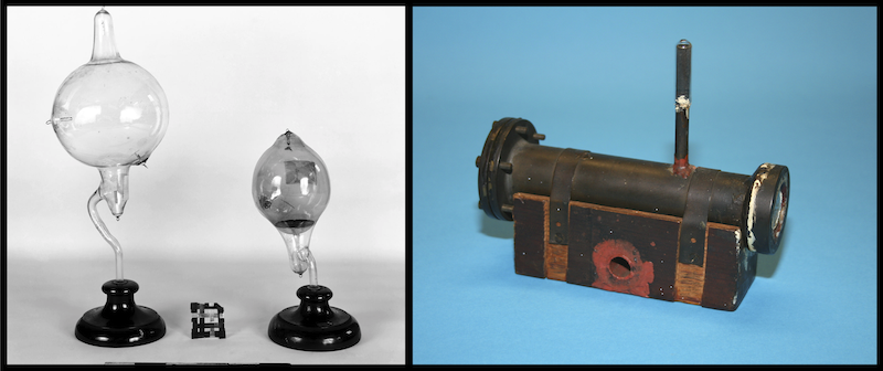
The first X-ray and neutron sources (developed by Röntgen and Chadwick, both of whom duly received Nobel Prizes for their discoveries) could fit on a desktop; examples are shown in Figure 1. Unfortunately, these historical apparatuses produce insufficient X-ray or neutron intensity for the kind of experiments that actually make use of the radiation. To enable these experiments, large-scale facilities have been built across the world, which produce much higher fluxes. For example, a next generation X-ray source will be 10¹⁵ times more brilliant than one of these historical X-ray tubes, and a new neutron source will have a flux 10¹⁸ times greater than that produced by Chadwick. The greater intensity of X-rays and neutrons generated at these large-scale facilities not only makes measurements possible but enables smaller and smaller samples to be analyzed at higher and higher throughputs.

Figure 1. Early apparatuses to produce X-rays and neutrons. (Left) Crookes tube with concave cathode, the early way to produce X-rays. (Image from the Science Museum Group Collection, copyright The Board of Trustees of the Science Museum) (Right) James Chadwick’s Neutron Chamber device. (Image from the Department of Physics, The Cavendish Laboratory, University of Cambridge)

Intense and well-defined X-ray beams are primarily produced by the acceleration of electrons in machines called synchrotrons, which emit X-rays when magnets are used to bend electrons as they travel around the ring. Neutron beams are produced either by a nuclear reactor or at a spallation source, which emit neutrons from a metal target that has been bombarded by high energy protons. None of these are on the scale of a typical laboratory though, and instead, they require large-scale facilities.

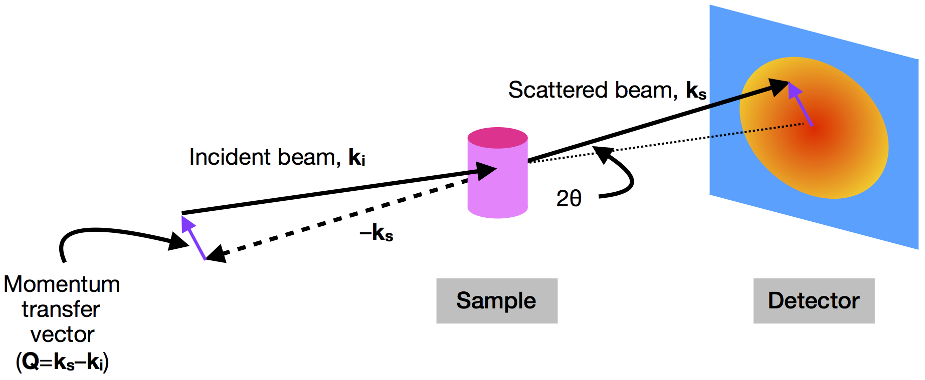
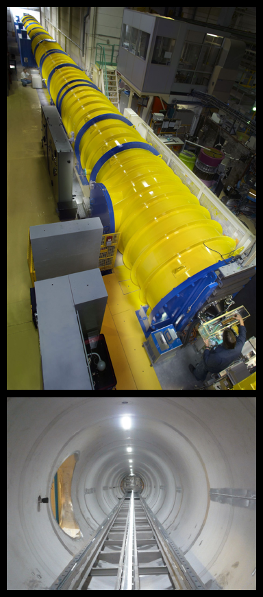
These large-scale facilities are definitely required for some small-angle scattering experiments. The larger a particle is, the smaller an angle that it will scatter at. Small-angle scattering measurements do indeed measure very small angles (less than 1°). This means that large distances between samples and detectors are required to measure scattering at these very small angles. There are instruments with 40 meter vacuum tanks and even 100 meter vacuum tanks. Examples of some long instruments are shown in Figure 2. This means that the size of the structures you are studying (ångströms, nanometers or micrometers) is very out of proportion with the size of the facilities you use (multiple meters).

Figure 2. Long instruments for neutron and X-ray scattering. (Top) The new 40m long detector tank of the small angle neutron scattering (SANS) instrument D11, at the Institut Laue–Langevin. (Image from Peter Lindner) (Bottom) Inside view of the 34 m detector tube at ID02 at the ESRF. The detector that measures scattered X-rays travels along the tube. (Image from T. Narayanan)

The ability of some instruments to access very long length scales from scattering at very small angles is the exact reason for my journey to the Advanced Photon Source (APS) near Chicago. For this experiment, I am interested in studying nanoparticles with diameters of several hundred nanometers but with interactions between particles that span distances much longer than this. To study interactions at the scale of micrometers, we need to measure scattering at the APS’s ultra-small-angle X-ray scattering instrument.

As you might guess given my long journey from Copenhagen to Chicago, there are a limited number of these instruments in the world. Even if there is a facility nearby, only a small number of samples can normally be measured rapidly, and even that might require waiting weeks or months. It is not possible to easily do test measurements at facilities, like you can with laboratory-based equipment. There are two ways to access time on these instruments, which as it is “time” on instruments using “beams” of X-rays or neutrons, is literally called “beamtime”.

Commercial access is more rapid, but it is costly (on the order of tens of thousands of dollars a day). Academic access costs less, and tends to be funded by the facility or a national fund, but you have to compete to get access this way. To gain beamtime via the academic route, I had to design and propose an experiment and have it accepted by a panel. Competing for and booking time at large-scale facilities is common in other fields, like astrophysics or particle physics. However, it is not typically necessary for soft matter experiments.

After being granted access by the panel for some beamtime on my desired instrument, the planning begins. The first thing to do is to schedule a time for the measurement with a local scientist at the facility. This might be during a weekend or a holiday, and I may have to be there overnight. I then need to update my radiation safety and awareness trainings and tests, which enables me to enter the facility, and book my travel. Finally, I prepare the samples, which I send to the facility a few weeks before my experiment. Once I arrive at the facility and familiarize myself with operating the instrument, I will finally perform my measurements. If all goes well, I will come home with a mountain of data to analyze. This time I am looking at nanoparticles, but depending on the materials I bring, I may reveal the structure of a protein or the size and shape of a micelle or the interactions between components in a complex mixture. There are a lot of possibilities in studying soft matter and biology. However, even if I haven’t found all the answers, I should hopefully have enough preliminary data to write my next proposal. This may sound like a lot of work, but given the capabilities available on the instruments at large-scale facilities, we can really push the limits of what is achievable in soft material characterization. There are over 100 neutron and X-ray facilities around the world, and one may be near you. If not, you too may get to travel thousands of miles for a brief window of beamtime.

The featured image at the top is an impression of Science Village Scandinavia, which is designed to surround the new MAX IV X-ray synchrotron and ESS neutron source being constructed in Lund, Sweden. (Image from COBE.)

We are surrounded by phenomena caused by the scattering of light. When enjoying a sunny day at the seaside, like in the photo at the top, why is the sky blue? Blue light scatters more than red light. Why is milk opaque? Protein and fat particles scatter light. If you are reading this with blue eyes, your eye color is due to light scattering. Scientists use the same general scattering principle to study the structure of soft materials using the scattering of well-defined radiation. Scattering measurements reveal structures between an ångström and hundreds of nanometers, an important region for studying soft matter. Just as the color of the sky results from light scattered by air molecules, the scattering of X-rays and neutrons tells us about the size and shape of compounds in soft materials along with their interactions, and I will focus on these two types of radiation.

In a small-angle scattering experiment (SAXS when using X-rays and SANS when using neutrons), a sample (whether solution, dispersion, or solid) is placed between an incoming beam of radiation and a detector (see Figure 1) [1]. The detector measures the scattering intensity as a function of angle, which in turn can be related to the size and shape of the sample’s components.

Scattering intensity is quantified as a function of the momentum transfer vector (or scattering vector) $\mathbf{Q}$ , which is simply the difference between the momentum of the incoming beam ( $\mathbf{k_i}$ ) and the scattered beam ( $\mathbf{k_s}$ ). The magnitude of $\mathbf{Q}$ (equal to $(4 \pi \sin{\theta}) / \lambda$ ) depends on the scattering angle ( $2 \theta$ ) and the wavelength of the radiation ( $\lambda$ ) [2].

Figure 1. The geometry of a small-angle scattering instrument. An incident beam of X-rays or neutrons (with momentum $\mathbf{k_i}$ ) is scattered by a sample with an angle of $2 \theta$ . The scattered beam (with momentum $\mathbf{k_s}$ ) is then detected at a point beyond the sample. The difference in momentum between the incident and scattered beams is $\mathbf{Q}$ . (Image produced by the author.)

Figure 1. The geometry of a small-angle scattering instrument. An incident beam of X-rays or neutrons (with momentum $\mathbf{k_i}$ ) is scattered by a sample with an angle of $2 \theta$ . The scattered beam (with momentum $\mathbf{k_s}$ ) is then detected at a point beyond the sample. The difference in momentum between the incident and scattered beams is $\mathbf{Q}$ . (Image produced by the author.)

The relationship between the magnitude of $\mathbf{Q}$ and the length scale being investigated ( $d$ ) is given by the equation $Q = 2 \pi / d$ , and this inverse relationship to distance is why measurements as a function of $Q$ are said to be in reciprocal space. (This relationship comes from Bragg’s law for crystals [3].) In real space, the arrangement of objects is described by the distances between them. In reciprocal space, the same arrangement would be given by $Q$ . The scattering process is essentially a Fourier transform [4], a mathematical procedure to convert waves to frequencies, making it possible to go between real and reciprocal spaces.

Now, having established some of the fundamentals of waves and scattering, we need to think about how radiation interacts with materials. This interaction determines the way that scattering data look and also what information you can obtain. Specifically, X-rays interact with electrons, and neutrons interact with nuclei. The magnitude of the interaction is quantified by the amount per volume (the “scattering length density”), and a difference in scattering length density between solutes and solvents results in detectable scattering. The scattering length density can be thought of as the “refractive index” for neutrons or X-rays. Figure 2 shows the general idea of contrast for any scattering experiment, with a comparison between homogeneous and heterogeneous solutes. When the color of the solvent and particle are the same shade of blue (meaning they have the same scattering length density), there is no scattering from that component. When the colors are different (meaning that they have different scattering length densities), there is now scattering.

Contrast schematic for homogenous and heterogeneous solutes — Figure 2. Schematic of how the contrast between solutes (circle) and solvents (surrounding) for solvents and solutes with different scattering length densities gives rise to scattering. When the two colors are matched, which is possible for homogeneous solutes (left), there is no scattering. For heterogeneous solutes (right), there is no one solvent that can match the entire particle. (Image produced by the author.)

Interactions between X-rays and materials are fixed by their composition. However, neutrons interact differently with different isotopes of the same element. One particularly useful difference, especially for soft organic materials, is for structures with protons (¹H) and those where protons are exchanged for deuterons (²H or D) [5]. It is possible to detect scattering from specific parts of complex systems by tuning the contrast of different components using solvents with different contrasts, as shown in Figure 2. Figure 3 shows calculated SANS (left) and SAXS (right) curves from chemically identical but isotopically distinct microemulsions, which are nanometer-sized droplets of water that are surrounded by surfactants in oil [6]. For the SANS curves, the dark grey areas represent deuterated oil or water (called D₂O or heavy water), and the light grey areas represent standard hydrogenous oil or water. Multiple contrasts are required for a heterogenous particle, because no single solvent can match the whole particle (Figure 2, right). The curves are all different, but the actual structure of the microemulsion is always the same. It is only the contrast that differs. A precise determination of the structural dimensions of the microemulsion can be determined by analyzing all the data together, which gives more certainty than considering any one alone.

Figure 3. Scattering intensity as a function of the $Q$ for water-in-oil microemulsions calculated for SANS (left) and SAXS (right). For the three SANS curves measured, the dark grey regions are deuterated water (D₂O) or deuterated oil, and the light grey regions are standard water (H₂O) or oil. For drop contrast (red), you detect surfactant and water. For core contrast (blue), you detect water only. For shell contrast (green), you detect surfactant only. For the SAXS curve (purple), the contrast is fixed, and the water core dominates. (Image produced by the author.)

Scattering data is analyzed by comparing experimental data to known equations for how different shapes should scatter radiation as a function of $Q$ . Luckily, many models are already known [7] for various shapes. However, as structures are determined somewhat indirectly from the scattering data, complementary information from other techniques, such as microscopy, is frequently obtained as well. The equation relating the shape and scattering as a function of $Q$ is called the “form factor”, an intraparticle property. For example, the curves in Figure 3 were all calculated using a form factor for a particle consisting of a spherical core surrounded by a shell of another material. At the extremes of $Q$ , approximations can be used to calculate the size (at low- $Q$ ) and the interfacial roughness (at high- $Q$ ). In addition, the size distribution usually must be considered. In the example in Figure 3, the radii of the cores do not have a single value. There is a size distribution of about 20%.

For more concentrated dispersions or for more strongly interacting systems, the interactions between the particles must be considered. In these cases, an interparticle property called the “structure factor” contributes to the shape of the scattering curves. It can be calculated for particles that are considered to interact as hard spheres, charged spheres, or attractive spheres. Often samples are studied dilute to avoid the structure factor contribution. However, for systems that are necessarily concentrated or charged, it must be accounted for.

In this post, I focussed on the fundamentals of scattering with examples from nanoparticle dispersions in dilute conditions. However, these are not the only kind of soft materials that can be studied. Polymer solutions and blends, complex fluids, liquid crystals, gels, and a variety of biological materials (such as proteins and nucleic acids in solution or lipid bilayers) can be studied using small-angle scattering. The properties of soft materials often emerge out of their structures. By characterizing them in a quantitative way, scientists can determine the relationships between structures and their functions. Using small-angle scattering, we can not only better understand materials but also better predict ways of improving them. Small-angle scattering should be one of the tools employed by everyone interested in soft materials.

The featured image at the top is a photo of Bellevue Beach in Klampenborg in Copenhagen, Denmark. (Image taken by the author.)

[1] A detailed discussion of detection and instrumentation is beyond the scope of this post, but the book chapter “Small-Angle Neutron Scattering and Applications in Soft Condensed Matter” is a great introduction if you are interested in learning more. ^

[2] The angles being scattered are truly small, typically on order of 1° or less. By using $Q$ , it is both the wavelength and angle that are important, and conveniently measurements performed using different wavelengths can be directly compared. ^

[3] Bragg’s law gives the conditions that a wave is diffracted by a series of planes. In a crystal diffraction measurement, peaks are observed in the data when Bragg’s law conditions are met. In a scattering measurement, where Bragg peaks are seldom observed, the relationship between $Q$ and $d$ is useful as a ruler for the length scale that is being examined. ^

[4] A Fourier transform is a mathematical operation that turns a periodic function, like a wave, into a probability of different frequencies. If, for example, you had a wave with a single wavelength, its Fourier transform would give a 100% probability at that wavelength. ^

[5] Deuterium is the heavy isotope of hydrogen with one neutron and one proton. ^

[6] A microemulsion is not just a small emulsion. Although, both are dispersions of two immiscible liquids, typically stabilized by a surfactant. A microemulsion is thermodynamically-stable and, in the case of a water-in-oil rather than oil-in-water, can be thought of as water-swollen surfactant micelle. Data for Aerosol OT-stabilized water-in-oil microemulsions can be found in the PhD thesis “Phase behaviour and interfacial properties of double-chain anionic surfactants” by Sandine Nave (University of Bristol). ^

[7] The equation for the scattering of a sphere was first given in the early 20th century by Lord Rayleigh who published this in the paper “The incidence of light upon a transparent sphere of dimensions comparable with the wave-length” in Proceedings of the Royal Society of London A in 1910. ^

Tag: neutrons

Small structures, Big facilities

Illuminating tiny structures: An introduction to small-angle scattering