Lifehack: How to pack two meters of chromatin into your cell’s nucleus, knot-free!

Original paper: The fractal globule as a model of chromatin architecture in the cell


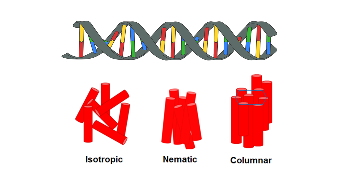
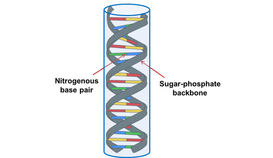
The entirety of our genetic information is encoded in our DNA. In our cells, it wraps together with proteins to form a flexible fiber about 2 metres long known as chromatin. Despite its length, each cell in our body keeps a copy of our chromatin in its nucleus, which is only about 10 microns across. For scale, if the nucleus was the size of a basketball, its chromatin would be  about 90 miles long. How can it all fit in there? To make matters worse, the cell needs chromatin to be easily accessible for reading and copying, so it can’t be all tangled up. It’s not surprising then that scientists have been puzzled as to how this packing problem can be reliably solved in every cell. The solution is to pack the chromatin in a specific way, and research suggests that this may be in the form of a “fractal globule”. 

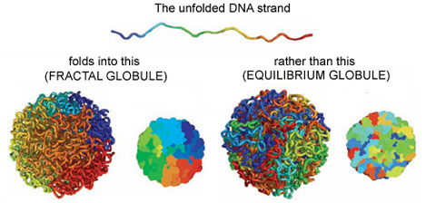
An equilibrium globule is the state that a polymer (a long repetitive molecular sequence, like chromatin) takes when it is left for a long time in a liquid that doesn’t dissolve it well. In such a liquid, the polymer is more attracted to itself than the molecules around it, so it collapses into a globule to minimize the amount of contact between itself and its surroundings. The resulting object is much denser than typical polymers in good solvents and is dense enough to fit inside a nucleus. However, like stuffing headphone cables into your pocket, it develops many knots and its different regions mix with one another.

On the other hand, if you change the polymer’s environment fast enough that it doesn’t have the time to fully equilibrate, then every piece of the polymer will locally collapse into its own globule. In other words, the polymer forms a globule made of smaller globules and is called a fractal globule. Fractals are objects which look the same at all scales, like the edge of a cloud or the coastline of England. If you zoom in or out on either of these objects, they look more or less the same. This isn’t an “equilibrium” state, meaning it will slowly fall out of this configuration. However, until the whole polymer equilibrates (which takes a long time), the chain has many desirable properties.

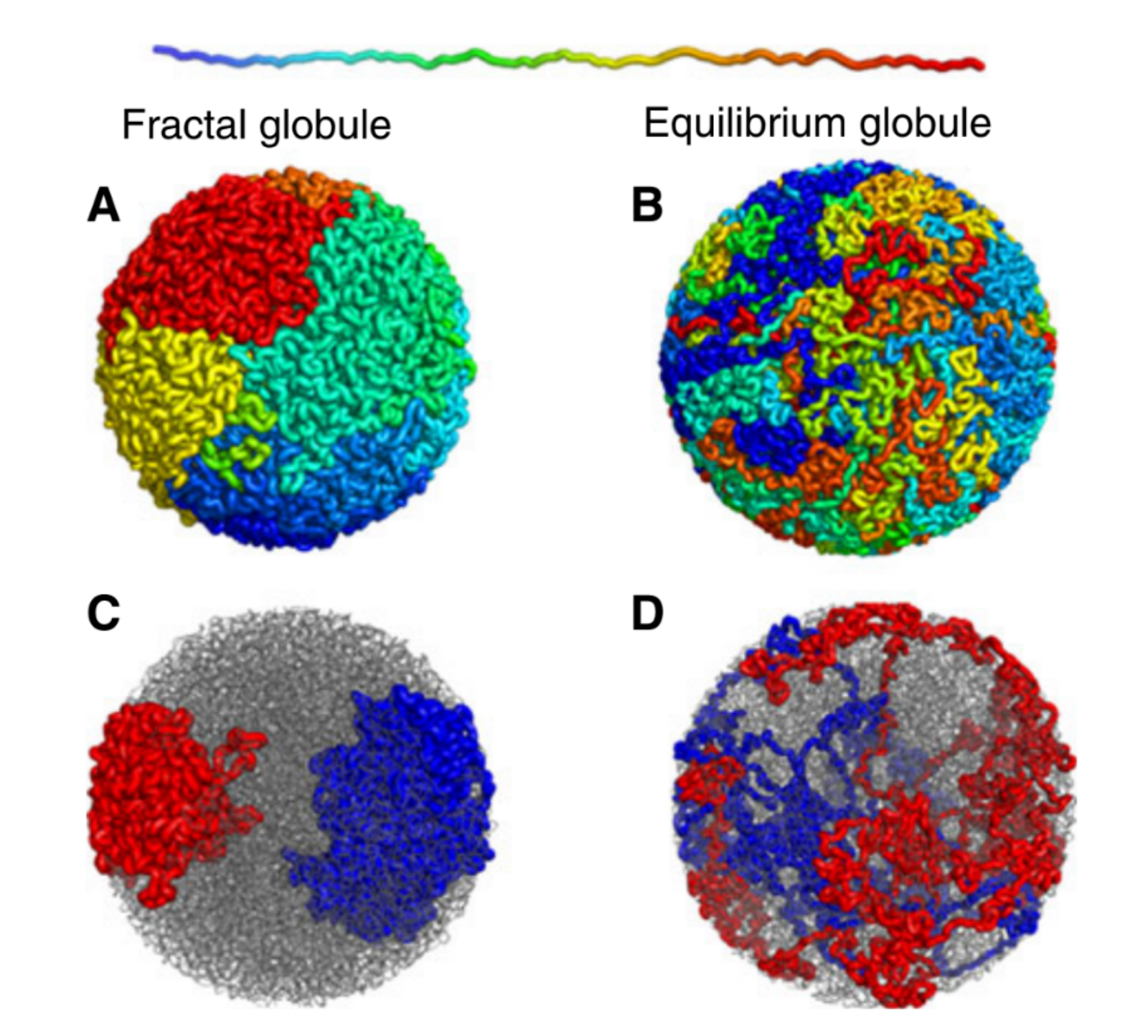
Figure 1. Simulated examples of fractal (A,C) and equilibrium globules (B,D), showing compartmentalization of different portions of the polymer. The chain color goes from red to blue as shown above. Compartmentalization means that parts of the chromatin stay near other parts with the same color (adapted from paper [1]).

We are interested in these globule states because they are dense enough that a globule of chromatin can fit inside of a cell nucleus. But it’s not enough to simply fit inside; the cell needs chromatin to avoid forming knots, since getting tangled would prevent the cell from properly reading its own DNA. Live cells also keep their chromatin nicely compartmentalized, that is, different regions along the genome stay spatially separated from one another. Unlike equilibrium globules, fractal globules have few knots and are also compartmentalized! To get a better picture for what this means, Leonid Mirny performed simulations of the different types of globules. Figure 1 shows the results of these simulations, highlighting how different the two states look in terms of knotting and separation of regions of the polymer. 

So it seems that the fractal globule state has all the properties we need for a good model of chromatin! But, as scientists, we know that no matter how well a theory fits the characteristics we want it to have, we need experimental evidence before believing anything. In the case of this fractal globule model for genome organization, evidence has come in the form of “contact probability maps”. These are collected from large populations of cells whose DNA is cut, spliced, and read in such a way that allows for a measurement of the probability that any two sites on the chromatin are touching at any given time. Among other things, these maps give us information about how chromatin is packed. So the question becomes, “what does the fractal globule model predict a contact probability map to look like?”

The fractal globule model doesn’t make exact predictions about where one will find specific segments of chromatin, but it does predict a contact probability as a function of distance between two sites, s. Specifically, the model predicts that the contact probability between two sites scales like 1/s. Meaning, if I look at sites that are twice as far apart along the polymer, then they are half as likely to be touching. This 1/s scaling is what was observed on intermediate scales (about 100,000 to 6 million base pairs) by looking at contact probability maps averaged over a whole population of cells.

We still don’t know how the cell maintains and tunes this fractal globule state, and we still have not developed a dynamic version of this picture, which is necessary since it is well-established that the chromatin in our cells is far from static. But this study gives us a new picture of how chromatin is organized inside cells. It isn’t randomly configured like headphone cables in your pocket or a ball of yarn. Rather it is folded onto itself in a self-similar way. This model is attractively simple, requires little fine-tuning, all while producing a long-lived state with segregated territories and easily accessible genes. 

[1] Mirny, Leonid (2011), The fractal globule as a model of chromatin architecture in the cell. Chromosome Res.

Featured image for the article is taken from Wikimedia Commons.

Researchers play with elastic bands to understand DNA and protein structures.

Topology, Geometry, and Mechanics of Strongly Stretched and Twisted Filaments: Solenoids, Plectonemes, and Artificial Muscle Fibers

Much of how DNA and proteins function depends on their conformations. Diseases like Alzheimers’ and Parkinsons’ have been linked to misfolding of proteins, and unwinding DNA’s double-helix structure is crucial to the DNA self-copying process. Yet, it’s difficult to study an individual molecule’s mechanical properties. Manipulating objects at such a small scale requires tools like optical and magnetic tweezers that produce forces and torques on the order of pico-Newtons, which are hard to measure accurately. One way around these difficulties is by modeling a complicated molecule as an elastic fiber that deforms in predictable ways due to extension and rotation. However, there are still many things we don’t know about how even a simple elastic fiber behaves when it is stretched and twisted at the same time. Recently, Nicholas Charles and researchers from Harvard published a study that used simulations of elastic fibers to probe their response to stretching and rotation applied simultaneously. The results shed light on how DNA, proteins, and other fibrous materials respond to forces and get their intricate shapes.

Before continuing, I would recommend finding a rubber band. A deep understanding of this work can be gained by playing along with this article.

Long and thin elastic materials, (like DNA, protein, and rubber bands), are a lot like springs. You can stretch or compress them, storing energy in the material proportional to how much you change its length. However, compressing them too much may make the material bend sideways, or “buckle”. It might be more natural to think of this process with a stiff beam like in Figure 1, where a large compressive load can be applied before the beam buckles. But since your rubber band is soft and slender, it buckles almost immediately.

A stick is compressed and at a certain pressure, buckles.
Figure 1. A straight, untwisted stick is compressed and buckles. It’s stiffer and thicker than your rubber band, so it sustains a higher load before buckling. (https://enterfea.com/what-is-buckling-analysis/)

Likewise, twisting your rubber band in either direction will store energy in the band proportional to how much it’s twisted. And, like compression, twisting can also cause it to deform suddenly. Instead of buckling, the result is a double-helix-like braid that grows perpendicular to the fiber’s length, as shown in Figure 2. An important caveat is that the ends of the rubber band are allowed to come together. But what happens when the ends of the band are fixed?

An elastic fiber is twisted into a plectoneme. It looks like a double-helix.
Figure 2. An elastic fiber is held with little to no tension and twisted. A double-helix, braid-like structure is formed. (Mattia Gazzola, https://www.youtube.com/watch?v=5WRkBWXUCNs)

Fixing the ends of a rubber band forces it to stretch as it twists. When this happens, a different kind of deformation can occur that combines extending, twisting, and bending the fiber. By stretching and bending simultaneously, the band forms a solenoid that is oriented along the long-axis of the band, reminiscent of the coil of a spring. An example of the solenoid shape appears in Figure 3.

An elastic fiber is held under tension and twisted. A solenoid structure is produced.
Figure 3. An elastic fiber is held at high tension and twisted. A solenoid structure is formed. (Mattia Gazzola, https://www.youtube.com/watch?v=0LoIwE37aNo)

All of the phenomena described above can be seen by playing with rubber bands, yet a quantitative understanding of how these states form and how to transition between them has remained elusive. To tackle this problem, Charles and coworkers used a computer simulation to calculate the energy stored at each point along an elastic fiber when it is stretched and twisted. The simulated fiber was allowed to deform and search for its lowest energy configuration, a process critical to navigating the system’s instabilities and finding the state you would expect to find in nature.

Figure 4 summarizes some of the different conformations attained by a fiber that is first stretched, then twisted to different degrees. We can see how a fiber with the same tension and different degrees of twist can lead to any one of a wide range of conformations. For instance, a fiber remains straight (yellow dots) when it’s stretched to a length $latex L$ that is 10% longer than its original length $latex L_{0}$ $latex (L/L_{0} = 1.1)$ until it is twisted by $latex \Phi a \approx 1$, where $latex \Phi a$ is the degree of twist multiplied by the fiber’s width divided by its length. Above this value of $latex \Phi a$, the simulated fiber twists into the braided helix structure seen in Figure 2 (blue dots). Likewise, when $latex L/L_{0} = 1.2$, the fiber remains straight until it has a much higher twist, $latex \Phi a \approx 1.5$, where it forms a solenoid (red dots).

Phase diagram of fiber conformations as a function of twist and stretch.
Figure 4. Conformation of a simulated fiber under constant extension $latex L/L_{0}$, twisted by $latex \Phi$ normalized by the fiber dimensions $latex a$. Orange dots are straight, blue dots are double-helix braids, red dots are solenoids, and green dots are mixed states. Black and grey symbols are experimental results from a previous study.

Considering the vast understanding of the universe that physics has given us, it may be surprising that there is so much left to learn from the lowly rubber band. While it’s fun to play with, understanding the way fibers deform could help researchers understand all sorts of biological mysteries. For instance, your DNA is a unique code that contains all of the information needed to create any type of cell you have, but depending on where the cell is in your body, that same DNA only makes some specific cell types. The cell can do this by selectively replicating sections of its DNA while ignoring others. One way it does this is by hiding away certain regions of DNA through folding. Exploring the way simple elastic fibers deform could help explain the way DNA knows how to make the right cells, in the right places.

Discovery of Liquid Crystals in Short DNA

Original paper: End-to-End Stacking and Liquid Crystal Condensation of 6- to 20- Base Pair DNA Duplexes


Ever since its discovery, scientists have known that the DNA molecule is present in every life form. It carries the genetic information of all living organisms and many viruses. Today, however, we will strip DNA of its genetic importance and look at it from a different perspective. We will discuss why DNA attracts attention even outside of the biological context: What is the connection between DNA and liquid crystals? What are end-to-end stacking interactions and why are they important? If you want to get answers on these questions (and many more), keep reading.

The chemical structure of DNA is intimately related to its geometry and physico-chemical properties. In water-based solutions, DNA is negatively charged. Since like charges repel, one DNA molecule pushes others away, effectively claiming  some  volume of space for itself [1]. Because electric repulsion decreases with distance, two DNA molecules cannot feel any kind of interactions when they are far away from each other. These features make it possible, together with DNA’s rod-like geometry, to model short DNA fragments (in this context, the term “DNA fragment” refers to an individual DNA molecule that’s much shorter than the length of a gene [2]) in a simplified way, as a hard repulsive rod (Fig.1.).

Fig1_png
Fig. 1. Structure of double-stranded DNA. Hydrophilic sugar-phosphate backbone is on the ‘outer’ side of the molecule, while hydrophobic nitrogenous bases are found on the ‘inner’ side. However, for simplicity, short DNA fragment is often modeled simply as hard repulsive rod (blue cylinder).

In the 1940s, researchers found that DNA molecules, when placed in solutions of water and salt, form liquid crystal (LC) phases. We all know the three phases of matter: gas, liquid and solid. LCs are substances that don’t fall into any of these categories. They are an intermediate phase that has properties of liquids as well as those of solid crystals — LCs can flow like liquids, but there is still some degree of order between the molecules. There are many types of liquid crystalline phases, the simplest of which is called the nematic phase. In the nematic phase, rod-like molecules (the “hard rods” of DNA in this case) point in the same direction on average [3]. This property gives nematic liquid crystals the ability to show colorful LC textures under a microscope equipped with a polarized light source (Fig. 2. b) [4].

According to theory, repulsive hard rods show the transition from a disordered fluid phase (called the isotropic phase) to the nematic LC phase only if they are sufficiently long and thin [1]. Almost 50 years later, Bolhuis and Frenkel confirmed this prediction by computer simulation [5].

In case of DNA, simulations predict that one shouldn’t expect to observe LCs for DNA fragments shorter than approximately 9 nm. So, when the authors of today’s paper observed LC textures in very short DNA fragments–  from approximately 2 to 7 nm — under a polarized-light microscope, it came as a real surprise.

Fig2_png
Fig. 2. a) With increasing concentration, a substance which shows liquid crystal behavior can undergo transitions between isotropic, nematic and columnar phase. b) Colorful textures of nematic liquid crystals visible under the microscope.

To understand this result,  let’s look in more detail at why hard rods in a solution begin to point in the same direction as their  concentration increases. In 1949, Lars Onsager published a paper in which he explained the entropic [1] origin of isotropic-nematic phase transition for hard rods. Entropy is usually understood as a measure of disorder. How then can the formation of liquid crystals lead to the increase of the total entropy in the system? To answer this question, we should understand the entropy as a measure of the number of possible configurations a system can have at a given state. According to Onsager, there is a balance between two contributions to the total entropy: while the number of different orientations available to each rod decreases in the process of ordering (decreased number of possible configurations), the centers of rods are able to move around more freely (Fig. 3.). The net effect is an increased number of possible configurations, which leads to an increase of total entropy in the system [6].

Fig3_png
Fig.3. Rods in a) parallel orientation and b) perpendicular orientation In the situation in (a), the rods are unable to rotate, but can translate (move in the way that all points of the rods move in the same direction and the same distance) freely, while in (b) the rods can rotate more feely but their translation is restricted.

The authors found that LC phases of short DNA share all the basic features of LC phases observed in long DNA fragments. As well as forming a nematic phase [3] at lower concentrations, with increasing concentration they undergo a transition to the columnar phase, where the molecules lie on top of each other in layers within which they often form hexagonal structure, as shown in Fig 2. a).

But how can LC ordering happen in  solutions of short DNA? It turns out that our simplified picture of DNA as a negatively charged rod was a bit too simple. To understand why, we need to learn a little more about the physico-chemical properties of the DNA molecule.  As shown in Fig. 1, the inside of DNA is made up of chemicals called nitrogenous bases. Like cooking oil or the surface of a teflon pan, these ‘water-fearing’ hydrophobic molecules tend to minimize their contact with water. However, at the terminal end of a short piece of DNA, some of the nitrogenous bases will be exposed to water. This is unavoidable — unless another DNA terminal end happens to be nearby. In that case, the ends tend to stick together to minimize their contact area with the surrounding water. This attraction between terminal ends of DNA is called the end-to-end stacking interaction and causes the formation of long, thin rods. And, as we already discussed, these rods are exactly the shape that gives rise to Onsager’s nematic phase.

If the main driving force for the formation of LCs in short DNA fragments is end-to-end stacking of terminal ends, the absence of these interactions should prevent LC ordering in the system. To disrupt end-to-end stacking interactions, authors chemically modify  their DNA fragments to disturb the attractive interactions between the terminal ends. By doing this, they can prevent the formation of LC phases in short DNA duplexes [7]. This experiment serves as another confirmation that end-to-end stacking interactions are indeed necessary to drive short DNA fragments to the formation of more ordered phases.

Fig4_png
Fig 4. End-to-end stacking of short DNA molecules  and the formation of nematic and columnar liquid crystal phases.

The research presented in this post provides a deeper understanding of the interactions that drive self-assembly of DNA and identifies a new type of interaction: hydrophobic end-to-end stacking between terminal ends of DNA. Identifying end-to-end stacking interactions represents another step towards better understanding of DNA as a generic (instead of genetic) building material and deciphering all of its unique properties.


[1] L. Onsager, Ann. N.Y. Acad. Sci. 51 (1949) 627-659

[2] For comparison, the smallest human genes, which are made up from DNA, are ‘only’ a few hundred nanometers long, while others are nearly a millimeter; every human cell contains approximately 2 meters of DNA in total.

[3] Double-stranded DNA is a chiral molecule with helical structure. For this reason, the nematic phase formed in solutions of DNA is called a  chiral nematic, and has different properties from a “plain-vanilla” nematic phase. However, this distinction is not relevant for us in this post.

[4]  Liquid crystals have the ability to change the direction of light polarization. This ability is called birefringence and it is responsible for the colorful textures of liquid crystals which we can observe under a microscope equipped with a polarized light source, but is also basic operating principle of modern TV and computer screens: Liquid Crystal Displays (LCDs).

[5] P. Bolhuis, D. Frenkel, J. Chem. Phys. 106 (1997) 666

[6] For further reading on this topic see: D. Frenkel, Nature materials 14 (2015) 9-12.

[7] M. Nakata, G. Zanchetta, B. D. Chapman, C. D. Jones, J. O. Cross, R. Pindak, T. Bellini, N. A. Clark, Science 318 (2007) 1276-1279

Knotty DNA

Original paper: Direct observation of DNA knots using a solid-state nanopore


Try taking out your earphones from your pocket and, in all probability, you’ll find knots and entanglements between the ends. As it turns out, this knotting effect is not limited to macroscopic objects, but occurs on the nanoscale as well. A DNA molecule that carries the genetic information of a living organism is actually a long string-like polymer, so you can imagine that it would also get tangled up just like the cords of your earphones. In fact, scientists know that DNA does form knots when it is in the nucleus of a cell, and these knots need to be removed by specialized bio-molecules, called enzymes, so that a cell can ‘read’ the genetic information encoded in the DNA. [1] In today’s paper, Calin Plesa and his colleagues at TU Delft are able to observe and measure these knots in DNA strands. In the process, they also observe interesting knotting behaviour which has not been observed before.

Knots on DNA

DNA translocation through a solid-state nanopore
Figure 1: This animation shows the DNA moving  through the nanopore. The associated dip in current is mapped onto the graph below. (Animation created by Calin Plesa, available under CC BY-SA license)

The researchers use a nanopore sensor to infer the structural properties of a DNA molecule. The sensor is made up of two reservoirs filled with electrolyte (a solution which separates into cations and anions, which can be used to conduct electricity, e.g. a salt solution), and they are separated by a membrane, or thin sheet, with a tiny hole in it. An electric field applied across the membrane generates an ionic current in the electrolyte and also pulls a negatively charged DNA strand through the tiny opening. The passage of a DNA strand through the nanopore causes a dip in the ionic current that is proportional to the volume of ions displaced—in other words, it’s proportional to the size of the molecule (a typical scenario is shown in Figure 1). Therefore, a knot in the DNA can generate a bigger drop in the current than an untangled strand. From this difference it is possible to infer the characteristics of the knot itself, since a bigger drop indicates a bigger knot.

The typical time for a DNA to pass through the pore is in the order of a few milliseconds, when the DNA is in a solution of potassium chloride (which is the typical salt solution used to carry out nanopore experiments). This makes it difficult technically, to see any features present on the DNA. Previous work has shown that it is possible to slow down the DNA passage by at least 10 times by using lithium chloride as their salt solution. [3] This increase in the translocation time (time it takes for the DNA to pass through the pore) is necessary to clearly see the additional dip in the current as the knot traverses the pore, as illustrated in Figure 2.

Translocation of a DNA molecule containing a trefoil knot through a solid-state nanopore
Figure 2: This animation shows a DNA with a knot moving through the pore. An additional dip in the current can be seen in the current trace as the knot (purple line) passes through the pore. (Animation created by Calin Plesa, available under CC BY-SA license)

The dip in the current signal caused by the knot passing through the pore can then be used to infer characteristics about the knot. In particular, it can be used to calculate the size of the knot, which has not been experimentally determined before. This has both physical and biological significance. Physically, it helps us understand the types of knots being formed on polymers as it can tell us whether the knot is loose or tightly formed. Biologically, it can help us understand how naturally occurring enzymes are able to disentangle knots in DNA strands, a function which is still poorly understood. The size of the knot is estimated by using

$latex d= v t$

where d is the length of the knot along the DNA strand, v is the average speed of the DNA translocation, and t is the time the knot takes to traverse the pore. Using this technique, the researchers estimate that the majority of the knots are less than 100 nm long. Previous research has shown that the DNA strand is rigid over lengths shorter than 50 nm, so considering this, the estimated knot size suggests that the knot is very tight. [2] However, this result needs further analysis, as the process of pulling the DNA through the nanopore might cause the knot to tighten, so this might not be the knot’s size in its natural state.

Slipping and sliding knots

When considering a linear (think: a thread with loose ends) DNA molecule, there is a possibility of the knot ‘slipping’ off the end of the strand before it gets pulled into the nanopore. For the knot to traverse the pore, it needs to be pulled fast enough to get squeezed to the size of the pore. If this process doesn’t happen fast enough the knot ‘halts’ at the pore entrance while the unknotted region translocates through. This allows the knot to disentangle, in case of a linear DNA molecule.

To determine if this slipping process occurs in knotted DNA strands, the researchers repeat their experiment using a circular (think: a thread joined end-to-end) DNA molecule. By using a closed loop they avoid possibility of the knot disentangling, but the knot can still slip towards the trailing end of the DNA during the translocation. The position of the knot is determined by the position of the dip in the current signal (purple line in Figure 2). They measure the probability of finding the knot at each position along the strand using two voltages, 100 mV and 200 mV. As shown in Figure 3, the knots show a preference for sliding toward the trailing end of the molecule at higher voltages, indicating that pulling too hard on the leading end of the DNA strand can indeed cause knots to slip along the strand instead of being pulled through the pore. The researchers also observe a 55% higher knotting occurrence in the circular molecules compared to linear ones. This suggests that knots may have slipped off the end of the linear molecules, thereby not detecting them at all.

Figure 4
Figure 3: The graph shows the probability of detecting the position of the knots along the length of DNA. At 200mV, the knots are observed to be at the trailing end of the DNA motion indicating the slipping phenomenon (adapted from Plesa et al.)

The researchers in this study have shown that naturally induced knots occur in DNA strands and they measured the sizes of those knots, which were previously unknown. This measurement showed that the knots detected are actually quite tight, which was not expected, although this result still needs to be investigated further. Additionally, these knots were seen to slide along the DNA molecules as they traversed the nanopore due to the strong pull at the end of the DNA strand. This was seen clearly by repeating the knotting experiments using circular DNA where there were no ends for the knots to slide off.

This new information about the structure of knots in DNA strands will help inform future studies of the complex topological structures formed in biomolecules such as DNA and proteins. It will also contribute to understanding the effects of topological features on the biological functions of these long, string-like biomolecules. In effect, it can help us explain the consequence of knotted DNA on the cell’s function as well as how the cell is equipped to handle these defects.

[1] http://www.tiem.utk.edu/~gross/bioed/webmodules/DNAknot.html

[2] Baumann, Christoph G., et al. “Ionic effects on the elasticity of single DNA molecules.” Proceedings of the National Academy of Sciences 94.12 (1997): 6185-6190.

[3] Kowalczyk, Stefan W., et al. “Slowing down DNA translocation through a nanopore in lithium chloride.” Nano letters 12.2 (2012): 1038-1044.