“I don’t think there will be a return journey, Mr. Frodo”: how thermodynamic irreversibility makes life flourish

Original paper: Statistical Physics of Self-Replication

Content review: Adam Fortais
Style review: Andrew Ton


Understanding the origin of life is one of the most enduring and fundamental scientific challenges there is. Of all branches of science, physics is probably not the first place one would think to go to for enlightenment. Life seems too complicated and multi-layered to be captured by the simplistic frameworks of physics. Today’s paper tackles a small part of understanding the origin of life – the physics of self-replication.

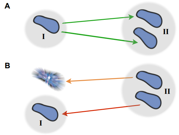
This paper begins by considering two macroscopic states, shown in Figure 1A, which are “one bacterium in a petri dish” and “two bacteria in a petri dish”, and considers transitions between these states. The biggest challenge here is relating a macroscopic change — the replication of a cell or collection of complex molecules — to a set of microscopic operations, also known as chemical reactions.  But these reactions are tremendously complicated. How can we know what to expect from them? The answer lies within the art of thermodynamics. 

Figure 1. Some of the pathways considered in the process of cell division. The probability of cell division (A) occurring is much higher than that of the disintegration of a single cell (B), highlighting the irreversibility of this event. Image courtesy of the original article.

According to thermodynamics, the governing quantities in a typical chemical reaction are energy, heat, and entropy. During a reaction, they can gain or lose any of these three as long as the total energy is kept balanced. Entropy, however, is a bit more special than the other two. Roughly speaking, entropy is a way of counting the number of possible ways a system can be in a certain state. So if a reaction involves several small molecules binding together to form a larger molecule, that involves a big loss in entropy. This is because there are many more ways to organize a large number of molecules than ways to organize one. Thermodynamics tells us that heat must be released to “pay for” this change in entropy. This heat flow increases the entropy of the environment, leading to an overall increase. All other things being equal, systems tend towards states of high entropy, simply because there are more ways of being in those states. This is usually referred to as the Second Law of Thermodynamics.

These are abstract descriptions of thermodynamic processes — how does the author use these to construct more concrete, quantitative models? First, they derive a version of the Second Law which relates the heat released by the transition to the irreversibility of the transition: the harder it is to undo a process, i.e. the more irreversible it is, the more heat must be released. Combining this observation with a simple model of replication, England reaches an important result: for a self-replicating system, the more efficiently it uses the available energy, the more rapidly it will replicate. 

England uses thermodynamics as a set of rules to calculate whether cell division for a bacterium is physically possible. While we already know the answer, the author is seeking to understand if this simple theory contains enough details to make accurate estimates about bacterial replication. The hard part of this problem isn’t to calculate the heat or entropy released, but rather to put a physical constraint on the likelihood of the reverse process. After all, we don’t ever see bacteria spontaneously dissolve back into their constituents. But with some clever thinking, this problem can be circumvented. Instead of considering the probability of a bacterium dissolving, the author simply considers the probability of every single chemical bond inside it spontaneously breaking. This is an extremely unlikely event, and yet it’s not as unlikely as the cell spontaneously being unmade, as shown in Figure 1B, and so it can give us a lower bound for the irreversibility of cell division. Combined with careful estimates of heat and entropy transfers, this gives a full (and very approximate) thermodynamic accounting of the process of cell division.

What can we do with this? We can perform some comparisons: first of all, the irreversibility of a process turns out to be a much larger thermodynamic barrier than the entropic difficulty of organizing all the constituents of a daughter bacterial cell, which is a highly structured object! This is surprising at first, but hindsight is 20/20: living systems are doing a lot of work to make things that don’t dissolve back into water. Another surprising conclusion of this argument is that real bacteria are tremendously efficient! With the coarse estimates used here, the author gets a replication rate close to that of a real E. Coli bacterium. This is an astonishing result, since the process considered here is not nearly as irreversible as that of a real cell division. 

The takeaway here isn’t simply learning something about bacteria or replication. The real lesson is about the power of the methods of statistical physics. The division of a bacterium is frighteningly complicated, and no physicist could write down the chain of reactions necessary for the proper replication and division of this complex system. Despite this intricacy, biological processes must still follow the unambiguous laws of physics. And that implies one thing: more life, more complexity, and more entropy. While this is by no means an answer to the question “where does life come from?”, it gives us hope that physics will continue to play an important role in the story of answering this question.

Who needs polymer physics when you can get worms drunk instead?

Original paper: Rheology of Entangled Active Polymer-Like T. Tubifex Worms (arXiv here)


If you speak to a soft matter physicist these days, within a few minutes the term “active matter” is bound to come up. A material is considered “active” when it burns energy to produce work, just like all sorts of molecular motors, proteins, and enzymes do inside your body. In this study, the scientists are focusing specifically on active polymers. These are long molecules which can burn energy to do physical work. Much of biological active matter is in the form of polymers (DNA or actin-myosin systems for example), and understanding them better would give direct insight into biophysics of all kinds. But polymers are microscopic objects with complex interactions, making them difficult to manipulate directly. To make matters worse, physicists have yet to fundamentally understand the behaviors of active materials, since they do not fit into our existing theories of so-called “passive” systems. In this study, Deblais and colleagues decided to entirely circumvent this problem by working with a much larger and easier-to-study system that behaves similarly to a polymer solution: a mixture of squirming worms in water.

The researchers focused on the viscous properties of this living material, which behaves somewhat like a fluid. Viscosity is a measure of a fluid’s resistance to gradients in the flow. Polymer fluids are highly viscous because the long molecules in a polymeric liquid get tangled up in one another. Physical descriptions of most fluids assume that viscosity is a constant (so called Newtonian fluids), but many materials exhibit what is called shear thinning. This is when a fluid flows more easily as one applies an increasing shear force, that is, a force pulling the system apart. We encounter shear thinning at the dinner table all the time when struggling to pour ketchup, another polymeric fluid, out of a bottle. If the bottle is shaken fast enough, increasing the shear force applied, the ketchup flows smoothly like a liquid. In polymer systems (like xanthan gum in the ketchup) shear thinning happens when polymers are pulled apart fast enough that they tend to align together, which loosens the entanglements that held the system together before. 

In this study, the researchers asked: how does shear thinning behavior change if the polymers in question were alive? To answer this question, they set out to measure the shear thinning properties of a mixture of worms at various levels of worm activity. Here, “worm activity” refers to how fast the worm is wriggling, which is calculated by measuring how quickly the distance between the two ends of a given worm changes. This leads to two logistical questions: how is the level of worm activity being modified, and how is the viscosity being measured?

Figure 1. This movie shows two worms, one in water (left) and one in a water + alcohol mixture (right). The worm on the right shows a decrease in activity when they are exposed to alcohol, which is one of the two ways the researchers modified worm activity in this study. Video taken from the original article.

The answer to the first question should be familiar to many humans. To make the worms less active, they were put into a solution containing water and a small amount of ethanol, the same type of alcohol found in beer, wine, and spirits. Once the worms were nice and drunk, the researchers noticed that they squirmed about more slowly, as shown in Figure 1. Thankfully, when the ethanol was removed, the worms returned to their previous level of activity! To make sure the alcohol wasn’t doing anything funny to the worms, they found a second way to reduce the activity — by reducing the temperature of the worm solution. Colder temperatures made for more chilled out worms, no pun intended.

Figure 2. This movie shows the functioning of the rheometer. The worms are placed inside a chamber between two plates. The top plate rotates with respect to the bottom plate, and the response of the material is measured. Video taken from the original article.

The researchers used a device called a parallel-plate rheometer to understand the shear thinning behavior of this living polymer system. As seen in Figure 2, a parallel-plate rheometer sandwiches a sample in between two flat plates and viscosity is measured by determining how much force is necessary to rotate the top plate, effectively pushing the material by twisting its surface. The viscosity of the worm mixtures was first determined at three different temperatures, and for worms drunk on ethanol. The results were surprising! The rheological behaviour of the low-activity worm mixtures matched with theories of polymer shear thinning quite well. It seems the worms have the same alignment properties as passive polymer solutions under shear!

So what happens when the worms are sober, more active, and wriggling around? They saw that the required twisting rate needed to thin the mixture decreased. In this case, the worm activity allowed for easier and quicker rearrangement while the mixture was pulled apart by the rheometer’s twisting motion. One can imagine that instead of needing to pull all the worms to the point of alignment, it may have been enough to nudge them in that direction and their wriggling did the rest. We can now imagine that the same thing might be true for non-living polymers: if a polymer material with shear thinning behavior is given an extra source of activity, then its thinning behavior may become more significant. 

The lesson to be learned here is partly about worms, polymers, and the adverse effects of ethanol, but really this experiment is a testament to the power and generality of physical descriptions. This study teaches us about the possible behavior of an active polymer system with processes that are relevant on the scale of a few micrometers, by studying real life worms that you can see with the naked eye! In general, it is usually possible to find analog systems that have the desired properties for your study, but which are easier to manipulate. Physics then gives you the bridge between the system of interest and your simpler analog, allowing you to harness the power of interdisciplinary science to ask questions previously unanswerable.

Featured image for the article is taken from the original article.

Lifehack: How to pack two meters of chromatin into your cell’s nucleus, knot-free!

Original paper: The fractal globule as a model of chromatin architecture in the cell


The entirety of our genetic information is encoded in our DNA. In our cells, it wraps together with proteins to form a flexible fiber about 2 metres long known as chromatin. Despite its length, each cell in our body keeps a copy of our chromatin in its nucleus, which is only about 10 microns across. For scale, if the nucleus was the size of a basketball, its chromatin would be  about 90 miles long. How can it all fit in there? To make matters worse, the cell needs chromatin to be easily accessible for reading and copying, so it can’t be all tangled up. It’s not surprising then that scientists have been puzzled as to how this packing problem can be reliably solved in every cell. The solution is to pack the chromatin in a specific way, and research suggests that this may be in the form of a “fractal globule”. 

An equilibrium globule is the state that a polymer (a long repetitive molecular sequence, like chromatin) takes when it is left for a long time in a liquid that doesn’t dissolve it well. In such a liquid, the polymer is more attracted to itself than the molecules around it, so it collapses into a globule to minimize the amount of contact between itself and its surroundings. The resulting object is much denser than typical polymers in good solvents and is dense enough to fit inside a nucleus. However, like stuffing headphone cables into your pocket, it develops many knots and its different regions mix with one another.

On the other hand, if you change the polymer’s environment fast enough that it doesn’t have the time to fully equilibrate, then every piece of the polymer will locally collapse into its own globule. In other words, the polymer forms a globule made of smaller globules and is called a fractal globule. Fractals are objects which look the same at all scales, like the edge of a cloud or the coastline of England. If you zoom in or out on either of these objects, they look more or less the same. This isn’t an “equilibrium” state, meaning it will slowly fall out of this configuration. However, until the whole polymer equilibrates (which takes a long time), the chain has many desirable properties.

Figure 1. Simulated examples of fractal (A,C) and equilibrium globules (B,D), showing compartmentalization of different portions of the polymer. The chain color goes from red to blue as shown above. Compartmentalization means that parts of the chromatin stay near other parts with the same color (adapted from paper [1]).

We are interested in these globule states because they are dense enough that a globule of chromatin can fit inside of a cell nucleus. But it’s not enough to simply fit inside; the cell needs chromatin to avoid forming knots, since getting tangled would prevent the cell from properly reading its own DNA. Live cells also keep their chromatin nicely compartmentalized, that is, different regions along the genome stay spatially separated from one another. Unlike equilibrium globules, fractal globules have few knots and are also compartmentalized! To get a better picture for what this means, Leonid Mirny performed simulations of the different types of globules. Figure 1 shows the results of these simulations, highlighting how different the two states look in terms of knotting and separation of regions of the polymer. 

So it seems that the fractal globule state has all the properties we need for a good model of chromatin! But, as scientists, we know that no matter how well a theory fits the characteristics we want it to have, we need experimental evidence before believing anything. In the case of this fractal globule model for genome organization, evidence has come in the form of “contact probability maps”. These are collected from large populations of cells whose DNA is cut, spliced, and read in such a way that allows for a measurement of the probability that any two sites on the chromatin are touching at any given time. Among other things, these maps give us information about how chromatin is packed. So the question becomes, “what does the fractal globule model predict a contact probability map to look like?”

The fractal globule model doesn’t make exact predictions about where one will find specific segments of chromatin, but it does predict a contact probability as a function of distance between two sites, s. Specifically, the model predicts that the contact probability between two sites scales like 1/s. Meaning, if I look at sites that are twice as far apart along the polymer, then they are half as likely to be touching. This 1/s scaling is what was observed on intermediate scales (about 100,000 to 6 million base pairs) by looking at contact probability maps averaged over a whole population of cells.

We still don’t know how the cell maintains and tunes this fractal globule state, and we still have not developed a dynamic version of this picture, which is necessary since it is well-established that the chromatin in our cells is far from static. But this study gives us a new picture of how chromatin is organized inside cells. It isn’t randomly configured like headphone cables in your pocket or a ball of yarn. Rather it is folded onto itself in a self-similar way. This model is attractively simple, requires little fine-tuning, all while producing a long-lived state with segregated territories and easily accessible genes. 

[1] Mirny, Leonid (2011), The fractal globule as a model of chromatin architecture in the cell. Chromosome Res.

Featured image for the article is taken from Wikimedia Commons.