Karen – Softbites

2019-10-10

The Future of Shape-Memory Polymers: Just Add Water and Glycerol

Original paper: Magnetically Addressable Shape-Memory and Stiffening in a Composite Elastomer

Video 1. Heat-shrink tubing demonstration.

Have you ever used heat-shrink tubing at home to seal an exposed wire? As shown in Video 1, you would place the tubing around your wire, apply heat, and voilà! The tubing shrinks and tightly wraps itself onto the exposed wire, and you don’t have to worry about an electric shock anymore. This type of material that changes its shape upon increased temperature is called a shape-memory polymer. Since its commercial development in 1962, scientists have found this type of material so useful that its popularity rose, especially in the biomedical and aerospace fields. However, it comes with a few drawbacks: applying the desired temperature uniformly can be tricky and the shape change induced by the heat can be quite slow. In addition, changing the temperature isn’t ideal for biological applications where the environment surrounding the material is sensitive to heat, such as in tissues and living cells. In today’s post, I’ll introduce you to a different type of shape-memory material that “remembers” its temporary shape when subjected to a magnetic field, instead of heat.

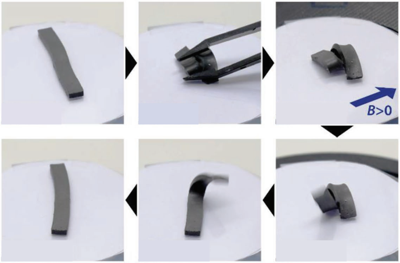
Video 2. Demonstration of the material developed by the authors.

Paolo Testa and coworkers from the Paul Scherrer Institute and ETH Zurich developed a shape-memory polymer composite that can preserve a new shape when a magnetic field is present. As you can see in Video 2, the initially flexible material sitting on the center stage is manually twisted with a tweezer and held by force. When the magnetic ring is raised around the stage and held up so that the material can “feel” the magnetic field, the material “freezes” in its twisted shape, even when the tweezer is removed. After a certain time, the magnetic ring is removed and the material regains its original shape within one second, dramatically faster than the time it took for a heat-shrink tubing in Video 1 to change its shape. The material—at least a part of it—that looks like black rubber is a flexible polymer that is the main ingredient of the Silly Putty, called poly(dimethylsiloxane) (PDMS). However, PDMS is normally transparent in color, and PDMS itself isn’t a shape-memory polymer. So what makes it black and capable of holding the twist when the magnetic field is present?

The answer is in iron particles. However, iron particles alone cannot perform well enough. Shape-memory materials that were previously developed had iron particles directly embedded in the polymer but didn’t have such a high sensitivity to magnetic fields. What makes the material in this paper so unique is the liquid surrounding the particles. The iron particles are dispersed in a water and glycerol mixture, making the fluid six times more viscous and stiff when subjected to the magnetic field. This type of fluid, called a magneto-rheological fluid, is then injected into the PDMS polymer, making the material sensitive to the presence of a magnetic field.

3D visualization of the material and 2D slices of that visualization with and without magnetic field — **Figure 1.** (a) 3D visualization of the PDMS injected with magneto-rheological fluid. (b)(c) 2D slices of a droplet surrounded by PDMS with the magnetic field (b) off and (c) on. (Adapted from the original paper.)

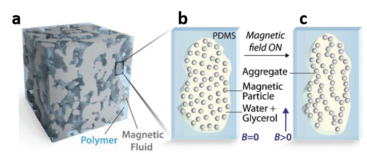
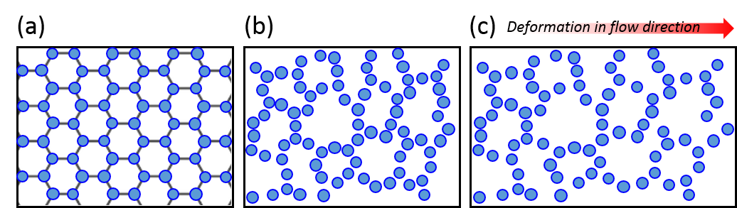
Figure 1 shows the 3D structure of the developed material, as well as a 2D schematic of a magneto-rheological fluid droplet with and without the magnetic field. When the fluid is injected into the polymer, the polymer encases the fluid and a composite is formed, which is shown in Figure 1a. In the absence of the magnetic field, shown in Figure 1b, the iron particles are dispersed and mobile inside the fluid droplet. However, when the magnetic field is turned on, shown in Figure 1c, the particles reorganize and align along the direction of the magnetic field, and, in turn, the droplet stiffens. The alignment of the iron particles and the resulting stiffening of the fluid, induced by the presence of a magnetic field, are the reasons why the polymer composite can hold its new shape (as in Video 2). When the magnetic field is removed, the particles regain their mobility and the fluid droplets soften, which lets the polymer return to its original shape.

On the left, a graph of stiffness as a function of the fluid volume fraction. In the middle, a graph of connectivity as a function of the fluid volume fraction. On the right, two 3D construction of material's internal structure, one representing 10% fluid and the other representing 40% fluid. — **Figure 2.** (a) The volume fraction (ratio) of magneto-rheological fluid over PDMS (?) versus the material stiffness. The blue and red lines indicate the magnetic field being on and off, respectively. (b) The volume fraction (ratio) of magneto-rheological fluid over PDMS (?) versus the connectivity between the fluid droplets. (c) 3D reconstructions of the material’s internal structure when the fluid occupies 10% (top) and 40% (bottom) of the total volume. PDMS and the fluid are represented in grey and red, respectively. (Adapted from the original paper.)

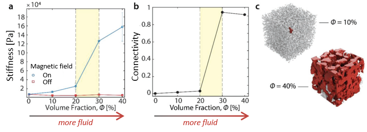
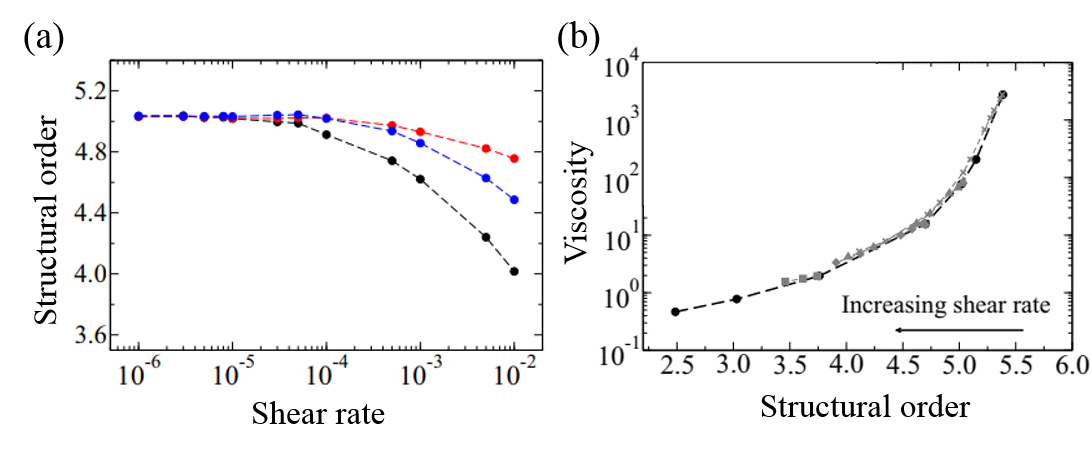
By controlling the ratio between the magneto-rheological fluid and PDMS (?), the authors tried to understand the relationship between the stiffness and structure of the material and the said ratio. When the percentage of the fluid increases, as shown in Figure 2a, the overall stiffness of the material measured in the presence of the magnetic field increases as well. This increase is enhanced when fluid occupies more than 20% in volume, as highlighted in yellow in Figure 2a. Compared to a factor of two increase going from 10% to 20%, the stiffness increases by a factor of 13 going from 10% to 30%.

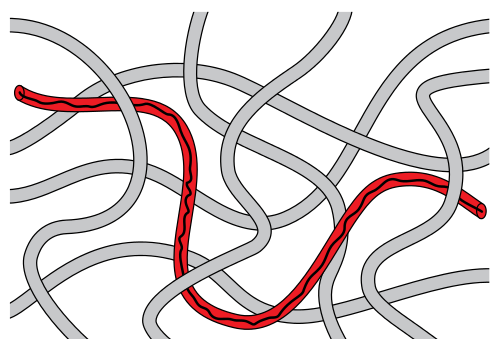
By measuring the connectivity [1] between the fluid droplets using an X-ray scan [2], the authors discovered that the stiffness increase is related to the network connection between the fluid droplets when the magnetic field is applied (Figure 2b). This network connection is visualized in Figure 2c; the fluid, shown in red, is isolated when the fluid composes only 10%. However, when increased to 40%, the dispersed fluid pockets become connected to one another, enhancing the stiffness of the overall material under the magnetic field.

As mentioned above, the addition of the fluid was the key to the material’s drastic functional improvement. Since the fluid provides freedom for the iron particles to move around and align under the magnetic field, the stiffening process becomes more dramatic compared to having the particles alone inside the polymer. Also, the fluid acts as a buffer, lessening any damages caused to the polymer by the motion of the hard particles. The authors hope that their research will open up an even wider range of applications using this shape-memory polymer, such as a magnetic-controlled micromachine that can deliver drugs to targeted areas inside our body. Unlike the temperature-controlled shape-memory material introduced in the beginning, the stiffening of this new magnetically controlled shape-memory material is reversible. This might offer a greater potential for new applications which might require several cycles of deformation. Maybe in the near future, we’ll use items made out of magnetically controlled shape-memory polymers in our daily lives.

[1] The connectivity is defined as the volume of the biggest droplet over the total volume of the magneto-rheological fluid in the polymer composite.^

[2] The authors used X-ray tomography, a method where a 3D image is constructed using 2D X-ray images.^

2019-05-08

Slithering Like A Snake and Beyond: Microscopy of Polymer Dynamics

Original paper: Entangled polymer dynamics beyond reptation

Scientists often draw inspiration from biological organisms to describe phenomena, even when they are studying outside the realm of biology. Physicist Pierre-Gilles de Gennes[1] was no exception. In 1971, after being inspired by the movement of snakes, he proposed reptation theory, or the reptation model, which has since been widely used to describe motions of polymers[2]. As the name “reptation” suggests, de Gennes assumed polymer chains move like snakes. As shown in Figure 1, the model describes a polymer chain’s motion in an environment that is highly populated by other chains (shown in gray) by assuming that the chain is confined in a virtual tube (shown in red) formed by surrounding polymer chains. According to reptation theory, the chain wiggles through this tube, similar to a snake slithering through the woods. As one might imagine, directly imaging the snake-like slithering of polymers is a challenging affair; however, in today’s study, Maram Abadi and coworkers from King Abdullah University of Science and Technology were able to do just that with DNA chains – an example of a polymer – and compared their results to prevailing theory.

**Figure 1.** A schematic of the reptation model. In a crowded and entangled polymer environment, a long and linear polymer chain (black) is located in a virtual tube (red), which traces the chain trajectory. Surrounding polymers are shown in gray. (Adapted from the Wikipedia page for reptation.)

While reptation theory has done fairly well in describing experimental observations of polymers, there are some shortcomings to both the experiments supporting this theory as well as to the theory itself. Namely, previous experiments mostly considered the overall motion of the chain; but local chain motion, such as motion at the ends of a polymer chain, have not been thoroughly studied. In addition, the theory was only designed for polymers with two ends, known as linear polymers. Thus, it does not account for the dynamics of polymers with different geometries, such as those that form rings, known as cyclic polymers. Given these observations, Abadi and coworkers realized that there was more work to be done in the studies of polymer dynamics.

To scrutinize the movements of the polymer chains, the authors used super-resolution fluorescence localization microscopy[3], which lets them monitor the movements beyond the typical microscopy resolution of ~200 nm. This technique allowed Abadi and coworkers to not only observe whole-chain dynamics but also local dynamics. To test the predictions of reptation theory, they chose both linear and cyclic DNAs with fluorescent dyes attached as model polymers for their study.

**Figure 2.** Fluorescent images of a linear DNA chain collected at different time points (indicated in the figure), overlapped for comparison. Insets show the enlarged views of the highlighted areas. (Adapted from the original paper.)

First, linear DNAs were used to confirm what has been known from reptation theory in great detail. Shown above in Figure 2 are images of a linear DNA as a function of time. Their results were consistent with theory. First, polymer chains traveled along virtual tubes that followed the contour of the chain (shown in white boxes in Figure 2A). Second, most of the polymer chain’s displacements were within the confinements of the virtual tubes, which had a diameter around 51–95 nm (shown in red boxes in Figure 2B). Further, they occasionally saw displacements of the DNA that exceeded the size of tube diameter (shown in cyan boxes in Figure 2C), known as constraint release in reptation theory. Finally, Abadi and coworkers observed that the chain-ends were able to move farther than the centers of the chains, which in turn creates a new tube for further DNA reptation (shown in green boxes in figure 2C). In reptation theory, this is called contour-length fluctuation.

However, there was one particular deviation from the theory found in the authors’ results. While the chain-ends were expected to move more freely than other parts of the chains, the chain-end motions were a lot faster than what is predicted by reptation theory. Therefore, the authors concluded that the motions at the chain-ends were beyond the scope of the reptation theory. These unexpectedly fast movements were not observed in previous experiments, in which only the chain as a whole was considered.

Fluorescent images of cyclic DNAs collected at different time points — **Figure 3.** Both rows are fluorescent images of cyclic DNAs collected at different time points (indicated in the figure), overlapped for comparison. 3A shows amoeba-like motion, and 3B shows contracting of an open structure. More details can be found in the main text below. (Adapted from the original paper.)

The authors also observed cyclic DNAs using the same methods. As they are not linear, reptation theory fails to accurately explain their movements. The authors observed diverse motion of the cyclic DNAs. You may notice in Figure 3A that the cyclic DNA has a loop-like region, shown in the white boxes. They found that cyclic DNAs repeatedly contract and extend this region, resembling the motions of amoeba. In addition, as shown in the first panel of Figure 3B, some cyclic DNA molecules may start with an open structure. However, as time progresses, these open DNAs may contract into more linear forms and expand back into the open shape again. Thus, Abadi and coworkers were able to show two phenomena that cannot be explained by reptation theory, thus requiring it to be further refined.

The results of this paper support many of the conclusions of reptation theory; however, it does suggest that there is still a need to expand this otherwise well-accepted theory. By considering different geometries and shorter timescales, this theory will be more powerful as a predictor or explainer of novel polymeric material dynamics. Furthering the understanding of polymer dynamics will then help us understand polymer properties for use in a variety of applications that we see in our lives every single day.

[1] This 1991 Nobel laureate in Physics is also the one who popularized the term “soft matter”.

[2] Polymers are molecules that are consist of repeating chemical structures.

[3] Super-resolution microscopy is a technique that lets us observe things that are smaller than the diffraction limit of ~200 nm, which is the limit that is imposed by the physics of light.

2018-12-052020-03-04

The Ketchup Conundrum and Molecular Dynamics: Unraveling the Mystery of Shear Thinning

Original paper: Structural predictor for nonlinear sheared dynamics in simple glass-forming liquids

We’ve all been there. We try pouring ketchup onto our fries from the bottle, but it doesn’t come out. So we tap the back of the bottle a few times, and suddenly, the ketchup rushes out and your entire meal is covered with it. Why does the ketchup exhibit such behavior?

This behavior is called shear thinning, and only some special fluids exhibit it. For fluids, such as water and alcohol (these are called “classical” or “Newtonian” fluids) viscosity only depends on temperature. Therefore, if the temperature doesn’t change, the viscosity remains constant (see the red curve in Figure 1). However, in non-Newtonian fluids, viscosity depends on another variable called the shear stress. Shear stress is the stress felt by materials when they undergo deformation caused by slip or slide. In shear-thinning fluids, which are a type of non-Newtonian fluids, the viscosity decreases when the shear stress increases (see the blue curve in Figure 1). Ketchup, with other suspension fluids such as blood and nail polish, falls into this category of shear-thinning fluids. So, by tapping the ketchup bottle, we apply shear stress to the ketchup inside, causing the viscosity to drop and making the ketchup flow out of the bottle. But, even though this phenomenon has been on scientists’ radar for a long time, the microscopic mechanism for shear thinning is still unknown for certain fluids.

**Figure 1.** Shear stress vs. viscosity of Newtonian and shear-thinning fluids.

Another type of fluid that exhibits shear-thinning behavior is the “supercooled” liquids. As shown in Figure 2, when a liquid – any liquid – is rapidly cooled below its freezing point, instead of crystallizing and solidifying (like what we typically see when water freezes in an ice-cube tray), it forms a supercooled liquid. When the temperature of this highly viscous liquids drops even further below its glass-forming temperature, it turns into a disordered glass-like phase [1]. That is why supercooled liquids are also called glass-forming liquids.

**Figure 2.** The relationship between the volume of liquid and supercooled liquid. *T_f* and *T_g* indicate freezing point and glass-forming temperature, respectively.

To understand the flow behavior of supercooled liquids, Trond Ingebrigtsen and Hajime Tanaka of the Institute of Industrial Science at the University of Tokyo ran molecular dynamics simulations. Molecular dynamics simulation is a computational method for studying the interactions of atoms or molecules. From the simulations, Ingebrigtsen and Tanaka were able to confirm what other scientists had previously suspected: shear thinning is linked to the increase in structural disorder of the liquid molecules (as illustrated in Figure 3(a) and 3(b)). To be more specific, it is linked to the structural disorder of molecules in the flow direction.

As a model for supercooled liquids, the authors chose to simulate a colloidal system, where molecules interact in a similar way to realistic fluids. After verifying that the simulates system acts like a supercooled liquid (for example, its viscosity decreases with increasing shear rate), they investigated the origin of shear thinning using this model. The molecular simulation revealed that as the shear rate increases, the molecular structure becomes more disordered. This is illustrated in Figure 3(a) and 3(b). More notably, the structural disorder was more prominent in the direction of the fluid flow compared to the structural disorder measured in any other directions relative to the flow. This can be seen from the black line of Figure 4(a), where the steep decrease of structural order could be observed with increasing shear rate.

Indeed, the structural disorder turned out to be the culprit behind the shear-thinning behavior in supercooled liquids. As shown in Figure 4(b), when the molecular structure becomes more disordered, the viscosity of the liquid decreases, a behavior expected in shear-thinning fluids. To understand this result, let’s picture molecules in the fluid. The shear applied in the direction of the flow would open up more space for molecules to rearrange themselves as the fluid expands, like it is shown in Figure 3(c). This leads to the decreased viscosity and the easier fluid flow.

**Figure 3.** (a) Structurally ordered molecular system. (b) A molecular system with increased disorder. (c) System after shear deformation in the flow direction.

**Figure 4.** (a) Shear rate versus structural order of the supercooled liquid model used in the molecular simulation. The black line represents the flow direction (blue and red each represents other two directions relative to the flow.) (b) Structural order versus viscosity. (Note the log scale on the y-axis.) All figures are adapted from the original paper.

This study sheds light on the previously unknown mechanism of shear thinning in supercooled liquids. Ingebrigtsen and Tanaka, however, insert that the microscopic mechanism for their observation should be further studied to fully understand the shear-thinning behavior. So, next time a disaster happens on your fries, chill out and think that you are just carrying out a super cool non-newtonian experiment!

(This post was updated on March 4th, 2020 to answer a comment that was made on the French translation of this post.)

[1] Technically, glass isn’t a phase, though I used that word for simplicity. Glass is an amorphous solid that has a disordered molecular structure (unlike ice, which has a well-defined crystalline structure). See Figure 3(b) for a visualization of a disordered molecular structure.