A Storm of Oscillators

Original paper: Oscillators that sync and swarm


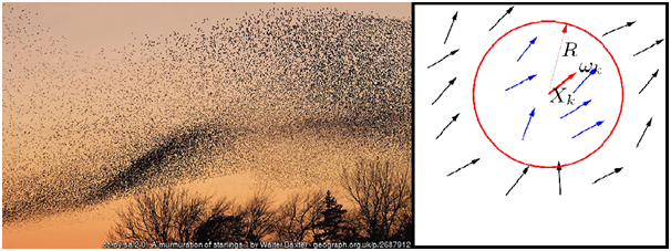
Japanese tree frogs follow a mating ritual that is so strange and beautiful that studying them may give rise to a new kind of science. During the rainy season, the male frogs gather near paddies and ponds and call to attract females. Researchers have found that isolated single male frogs call periodically [1], however, groups of males that are located near each other try to call out of sync. This temporal difference in calls allows the female frogs to correctly locate the male frogs. This is a natural system where spatial location of the frogs dictates the synchronization of their calls. This leads to an interesting question: What happens if you allow the synchronization of their calls to dictate their locations instead?

Scientists study synchronization to understand how an oscillating system evolves over time. However, systems ‘in sync’ do not usually move through space in a way that is related to their oscillations – consider the light flashes from a gathering of fireflies or the beating of a cardiac pacemaker. Swarming, on the other hand, is a form of self-organization where the participating individuals move through space, guided by some simple rules. In today’s paper by O’Keeffe, Hong, and Strogatz, the authors try to get a theoretical understanding of systems that show both synchronization and swarming. Previously, there had been studies of “mobile oscillators” where it was assumed that the location of an oscillator in space affected its phase. Here, the authors come up with a new theory that the phase affects where the oscillator is located in space. They name such particles swarmalators and propose a simple model to study their collective states analytically.

Imagine a set of particles on a plane, where each one is labeled by a number 1,2,3, etc. The ith particle (where i is any of the labels 1,2,3, etc.) has an internal state represented by a variable theta, $latex \mathbf{\theta}_i$, and a position represented by the vector $latex \mathbf{x}_i$. The internal state $latex \mathbf{\theta}_i$ is equivalent to a phase angle, so it can only take on values between 0 and 2?, while $latex \mathbf{x}_i$ can be any position on the plane. The key to swarmalators is that their position affects how their internal state changes and their internal state affects how their position changes. A relatively simple way to model this would be by the following set of equations:

$latex \dot{\mathbf{x}}_i =  \frac{1}{N} \sum_{j \neq i}^{N} \frac{x_j-x_i}{|x_j-x_i|}(1+J cos(\theta_j-\theta_i)) – \frac{x_j-x_i}{|x_j-x_i|^2}$

$latex \dot{\mathbf{\theta_i}} = \frac{K}{N}\sum_{j \neq i}^{N}\frac{sin(\theta_j-\theta_i)}{|x_j-x_i|}$

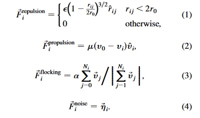
The most interesting parameters in these equations are J and K. Let’s step through the equations to see what their effects are. The first equation says how the position of the ith swarmalator changes in time, given by the time derivative of $latex \dot{\mathbf{x}}_i$. It is affected by all the other particles. The first term in the sum is an attraction between particles and points in the direction from particle i to particle j. The parameter J controls how oscillations lead to reorganization in space. For positive J, the closer two swarmalators internal states are, the more they attract since cos(x) is maximized around x = 0. When J is negative, swarmalators are attracted to swarmaltors with as different from an internal state as possible. When J = 0, swaramalators’ spatial movements are immune to other’s internal state. The second term is simply a repulsion between particles, preventing them from occupying the same place.

Similarly, the second equation says how the internal state (the phase angle) changes in time. Like the position, it has a constant angular velocity, $latex \mathbf{\omega}_i$, and is also affected by all the other particles. The parameter K represents how well the internal state of oscillations are synchronized for swarmalators. For a positive K, the swaramalators want to be synchronized with each other, while for negative K they want to oscillate out of phase. This effect is distance dependent, so swarmalators are more affected by nearby swarmalators than ones that are further away.

The authors use a computer to solve this pair of governing equations to see how such a system will evolve over time. They report that there can be five different states based on the two parameters J and K (Figure 1).

41467_2017_1190_Fig1_HTML
Figure 1: Diagram showing the various combinations of J and K which give rise to the various states of the model.

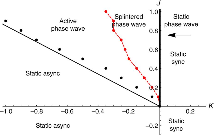
Static synchrony: For all positive K and all J, the model predicts that swarmalators will arrange themselves in a circularly symmetric manner. Each of the swarmalators will be fully synchronized in phase (Figure 2). All static states reach an equilibrium after some time.

41467_2017_1190_MOESM4_ESM
Figure 2: This animation shows the time evolution of swarmalators when they are in a state of static synchrony. All swarmalators occupy a disk and they all have the same phase.

Static asynchrony: For negative J and negative K, i.e. for cases when swarmalators want to oscillate out of phase but are attracted to opposite phases spatially, they are distributed uniformly and every phase occurs everywhere. (Figure 3).

41467_2017_1190_MOESM5_ESM
Figure 3: The animation shows how swarmalators evolve and rearrange themselves in the state of static asynchrony. The swarmaltors all occupy a disk, with phases different from their neighbors, leading to all phases existing everywhere.

Static phase wave: For the special case K=0 and J>0,.when the swarmalators’ phases are frozen in time but they like to settle near other swarmalators with the same phase, an interesting phenomenon occurs. Since positive J means “like attracts like” the swarmalators arrange themselves in regions of similar phases. This leads to an annular structure where the spatial angle of each swarmalator is perfectly correlated with its phase of oscillation (Figure 4).

41467_2017_1190_MOESM6_ESM.gif
Figure 4: The state of static phase wave where the spatial angle of the swarmalators is directly correlated to their phase of oscillation.

Splintered phase wave: In the K<0 half-plane, and when the magnitude of K is not too large, the swarmalators tend to oscillate out of phase weakly while trying to get closer to similar phases and a non-stationary state occurs. Here the particles keep rearranging themselves into disconnected clusters of distinct phases. Unlike the earlier static states, within each cluster, the swarmalators execute small amplitude oscillations in both position and phase about their mean values.

41467_2017_1190_MOESM7_ESM.gif
Figure 5: The splintered phase wave state.

Active phase wave: On decreasing K further — that is, when swarmalators strongly desynchronize but try to move towards swarmalators in sync — the oscillations in phase and position increase until the swarmalators start to execute regular cycles. Although this is a new phase, the authors point out that the motion of swarmalators is reminiscent of the double milling of biological swarms where the population splits into groups that are rotating in opposite directions.


41467_2017_1190_MOESM8_ESM.gif
Figure 6: Swarmalators showing an active phase wave.

In this paper, O’Keeffe and his colleagues have demonstrated how a system of particles that have the freedom to move in space and match the oscillation phase of their neighboring particles can lead to a rich variety of patterns that change in space and time. Perhaps most interestingly,  the authors claim that there is no known natural system where splintered phase waves and active phase waves occur. Thus, this paper provides an interesting lead for experimentalists searching for new patterns in nature.


[1] Mathematical modeling of frogs

Maxwell-Boltzmann in the Mosh Pit

Original paper: Collective Motion of Humans in Mosh and Circle Pits at Heavy Metal Concerts


You must have observed a flock of birds or a school of fish form wonderful patterns. The entire group behaves like one big organism. Have you ever wondered if humans behave similarly when many of them get together? Are there similarities between violent mobs or cheering crowds and a herd of sheep or a flock of birds? Today’s paper studies human behaviour in one such form of gathering – A mosh pit!

Before jumping into a mosh pit, it is worthwhile to discuss how systems made up of a collection of moving objects form complex patterns. One type of system where complex patterns arise occurs when each moving unit in the system interacts with its neighbours while maintaining the same absolute velocity. Systems of this sort are very common in biology, from schools of fish to flocks of starlings and swarms of locusts. In all these examples, each moving unit rarely communicates with the entire group to coordinate their motion. However, each individual in these groups is trying to move in the general direction of their nearest neighbours, and with the same speed as them. Tiny errors may occur while trying to follow the neighbourhood. Under the right circumstances, these tiny errors can give rise to complex patterns. This phenomenon, where patterns emerge because self-propelling particles try to align with their neighbours, can be modelled by a set of very simple equations introduced by Tamas Vicsek in 1995. This is one of the simplest models physicists use to study how patterns emerge in flocks.

1
Figure 1: Left: Starlings in flight form patterns. Flocking of birds is an example of collective motion where patterns emerge because each bird in the flock tries to follow in the general direction of their neighbours. Right: A bird labeled $latex k$ with position $latex X_k$ and velocity $latex w_k$ tries to align with the mean velocity of its neighbours within the disk of radius $latex R$

Human beings are capable of intelligent decision making on their own. Yet a crowd’s behaviour may not have any trace of the intelligence of an individual. Spontaneous formation of lanes of pedestrians, jamming during a panic-induced motion of a crowd and Mexican waves (also known as ‘the wave’ in the US) of cheering fans during a football match are all collective behaviours in response to stimuli from the surroundings. It is worth asking if the equations that describe the motion of flocks of birds can be applied to a collection of humans with reasonable accuracy.

In today’s paper, Silverberg and his colleagues study the dynamics of the crowd in heavy metal concerts. They study YouTube videos to calculate the speed distribution in mosh pits. While they refer to previous studies of crowd dynamics, they start this paper with a few surprising observations. Even though the density of people in a mosh pit is much higher than gaseous systems, their behaviour resembles gaseous particles. They report that the speed distribution in mosh pits fits well with the 2D Maxwell-Boltzmann distribution.

mbdist
Figure 2: An example of the Maxwell-Boltzmann distribution of speed of particles in a gas.

The Maxwell-Boltzmann distribution is used to describe the probability that a particle in a volume of gas moves with a certain speed. Such a distribution occurs when a volume of gas is in thermal equilibrium, meaning that the gas has the same temperature as its surroundings and its temperature does not change with time. The shape of that distribution suggests that there is a range of speeds, in the middle of the distribution, that includes the majority of the particles (denoted by the light blue bars in Figure 2). A much smaller fraction of particles is likely to move very fast or slow. Similarly, a small fraction of the participants in a mosh pit moves very fast, while the majority moves at a much slower pace.

A mosh pit resembles gaseous systems in equilibrium although it has all the characteristics of a non-equilibrium system –  it continuously changes with time as participants join or leave the pit, it changes shape on the suggestion of the performers on stage. Although it may be expected that each participant in a mosh pit moves with similar velocity as their neighbour, the authors show that there is no such dependence beyond one shoulder length. Thus it is not necessary that your neighbours have the same velocity as you, in a mosh pit. The authors go on to ask and answer the question: “why does an inherently non-equilibrium system exhibit equilibrium characteristics?”

3
Figure 3: The forces that can be used to describe the motion of crowds in a mosh pit. The repulsion force occurs due to collision and does not exist beyond two human shoulder length. The propulsion force describes the individual velocity and the force needed to move against or with the crowd. The flocking force describes the tendency to follow in the average direction and speed of the crowd. Noise term is used to quantify any other random behaviour.

They simplify the complex dynamics exhibited in a mosh pit by breaking it down to a few phenomena that can be observed intuitively. They observe that a mix of forces that describe repulsion due to collision, self-propulsion, flocking interaction and some random noise, can model the crowd.

Using these equations and suitable parameters, they simulate the dynamics of the crowd (Figure 4). It is interesting to note that the equations lead to three major phenomena that may dominate at various time scales. They are flocking, noise and collision. Noise and collision tend to disrupt any patterns, whereas the tendency to form flocks and follow the neighbours creates patterns. If it takes a long time to form flocks, the disruption from collisions and noise gives rise to random motion. Random motion has the nice property of making its velocity distribution look like a bell curve, which gives rise to the Maxwell-Boltzmann distribution[1].


circlepit
Figure 4: This is an example of a simulation of the crowd using the equations in figure 3. Red dots represent active participants who move around and thus experience flocking interactions. Black dots represent participants who prefer to remain stationary and are not subject to flocking interactions or random forces. This simulation can be accessed at: http://mattbierbaum.github.io/moshpits.js/


Therefore, a majority of random movers have a speed around the most probable one, whereas a tiny fraction moves fast or slow. This is similar to gases in equilibrium and answers the question why mosh pits that seem to be out of equilibrium behave like particles in an undisturbed gas. If, however, people form flocks faster than they collide with each other they tend to separate themselves out from non-participants. In this case, the flocking dominates for the active participants leading to a different distribution. The active participants are confined but they can move with a large angular momentum.

While studying human behaviour is a fun exercise, the authors conclude that such studies may help design better crowd management strategies and architectural safety protocols. Heavy metal concerts put a large number of humans in extreme conditions thus creating an opportunity to study how humans behave as a group.

[1] Vicsek, T. & Zafeiris, A. Collective motion. Phys. Rep. 517, 71–140 (2012).

[2] Simulation can be found at: http://mattbierbaum.github.io/moshpits.js/


1. The Gaussian distribution, or bell curve, describes the velocity of particles in a gas. The Maxwell-Boltzmann distribution for the speed (= absolute value of the velocity vector) can be derived from the Gaussian distribution of the velocities. (Link to: Distribution for the velocity vector)